Architecture
Not only are signal curves represented in the TwinCAT 3 Scope View; recording configurations are also created. For the creation of these configurations it is important to be familiar with the architecture of the TwinCAT 3 Scope View. This is reflected in the tree structure of the measurement project in the Solution Explorer. By right-clicking on the tree node, context menus can be opened with which various Scope functions can be called up, such as opening a window or adding elements below the selected node.
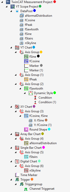
| Main level, at which several Scopes can be added. The Scopes within a project can be controlled independently of one another. | |
| A Scope always stands for a recording configuration. This means that all elements inserted below it are subject to the same recording settings. If a Scope is selected, the setting options such as recording time and ring buffer are displayed in the Visual Studio Properties window. See also: Scope node | |
| All raw acquisitions whose data are to be recorded are located in the DataPool. Whether they are displayed in the View as graphs depends on the configuration of the charts. A distinction is made between raw acquisitions and interpreted acquisitions | |
| Several YT charts can exist in parallel in a Scope. They are the actual display area in the view and provide the time base. Each chart has its own toolbar for changing the display. The color and axis settings can be made in the Properties window. Clicking on the signal curve in the chart highlights the respective channel in the Solution Explorer. See also: YT chart properties | |
|
| A chart (YT, XY, array or single bar) can have several axes. An axis provides the value range for the connected channels. Amongst others, the automatic or free scaling can be set in the Properties window. See also: YT axis properties |
| A channel represents the style characteristics of a selected variable. In the Properties window the color, marks and other parameters can be set. Double-clicking on the channel highlights the respective signal in the chart. | |
| The acquisition contains information on the actually selected variables. | |
| Markers are hierarchically assigned to the charts. X and Y markers can be added within a chart. Amongst other things, the current values of the signal/marker intersection and differences to the other markers are displayed in the Marker Tool window. Any desired number of X and Y markers can be set. See also: Marker | |
|
| With the help of Dynamic Styles, the style properties such as graph thickness or graph color can be changed at runtime based on the states of the same or other acquisitions. |
| Several XY charts can exist in parallel in a Scope. They represent the actual display area in the view. Each chart has its own toolbar for changing the display. The color and scaling settings can be made in the Properties window. Clicking on the signal curve in the chart highlights the respective channel in the Solution Explorer. See also: XY chart properties | |
|
| Shapes are geometric figures that can be placed in the charts. The figures can be individualized accordingly through the specification of coordinates. |
| An array bar chart can connect to an array in the controller and display each array element as a bar. Several array bar charts can exist in parallel in a Scope. The settings for the chart can be made in the Properties window. | |
| The bar chart displays a single variable as a bar diagram. The settings for this chart type can be made in the Property window. | |
| The Digital Chart displays one value per channel. In the Digital Chart the values are shown in a numerical display and axis groups can be used to group the channels. See also: Digital Chart properties | |
| Triggers are assigned to the Scopes in the tree structure of the Scope View. The trigger action, e.g. a Stop Record, can be set in the Properties window of the Trigger Group. The lower-level triggers can be logically linked to form a trigger condition. The variable selection also takes place here in the Properties window. See also: Trigger properties | |
 Measurement Scope Project
 Standard Scope Project
 DataPool
 YT Chart
 Axis
Axis Channel
 Acquisition
 Marker
 Dynamic Style
 XY Chart
 Shapes
 Array Bar Chart
 Single Bar Chart
 Digital Chart
 Trigger
The interfaces for the control of the Scope View are divided into several individual windows (Tool windows) and their position and size are freely configurable.
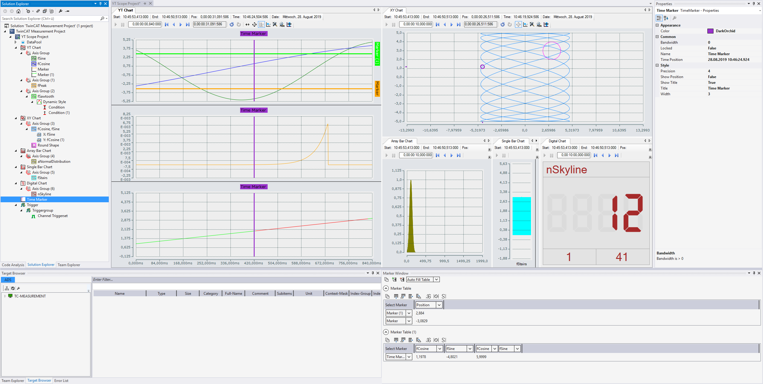
Solution Explorer | Display of the project structure within a solution. See also: Architecture |
Markers | Display of the values present at the X/Y-marker. See also: Markers |
Target Browser | Channels can be added to a Scope configuration via their symbol names using the Target Browser. See also: Target Browser |
Properties | The settings of the element marked in the Solution Explorer are displayed in the Properties and can be edited. See also: Scope nodes |
Error list | List of errors, warnings and messages. Each scope project lists the generated messages independently here. The messages for the respectively selected Scope can be deleted via the context menu command Clear Error List. |
ScopeViewControl | Display of the individual charts. The charts can be displayed next to each other or in overlapping tabs within the control, exactly like all other windows. |