Frequency analysis

Motivation

One of the most important methods in the diagnostic/analytic machine monitoring is the recording of vibrations with accelerometers and a frequency analysis based on that. The reason is that machines are made of metal and thus of elastic structures that are virtually always subjected to periodic forces. This leads to vibrations in which the frequencies and excitation forces and the characteristic frequencies of the respective structures are reflected. Vibration measurements therefore enable conclusions to be drawn regarding the structures and forces in the machine. Damage and structural changes of machine elements, such as bearings, result in changes to the vibration pattern.

The vibrations propagate in the machine components in the form of sound waves (structure-borne sound). As machines consist of a large number of parts, which transmit vibrations elastically to other components on the one hand and oscillate themselves on the other, filtering and superimposition of the individual vibration components occur. A vibration signal correspondingly consists of several signal components which, with different time delays and attenuations that depend on the distance traveled, add up to the total signal. Individually sought vibration components are therefore no longer recognizable in the time sequence of the total signal without further processing. The power of frequency analysis is that it can split the linearly superimposed vibrations into frequency components. These frequency components can then be more readily allocated to a particular machine state, component or process.

The concept of frequency-selective monitoring of components is divided into:

• Calculation of the spectrum
• Statistical assessment of the result
• Threshold value monitoring

Practical elements of the frequency analysis

The main aspects of the Fourier analysis have already been dealt with in the section Fourier analysis. At this point we will look again at the most important practical aspects.

In designing the parameters of the function block for Fourier analysis (e.g. FB_CMA_MagnitudeSpectrum or FB_CMA_PowerSpectrum), the following questions are of paramount importance.

• How high is the maximum frequency that is to be analyzed?
  The sampling frequency – via the terminal's oversampling factor – and the associated task cycle time are to be set accordingly. Attention must also be paid to the setting of an anti-aliasing filter. See section Samplinig theorem.
• What are the requirements for the frequency resolution?
  The length of the measuring time (size of the input array) must be set accordingly; see Frequency resolution. The deterioration of the frequency resolution when applying a window function should also be taken into account, see Window function.
• The FFT length must be larger than the length of the input array, and it must be a power of two. The surplus elements are filled with zeros; see Zero Padding or Frequency resolution.
• Suitable scaling of the spectrum must be selected, see Scaling of spectra.

The above points refer in particular to the use of the FB_CMA_MagnitudeSpectrum and FB_CMA_PowerSpectrum. When using special variants of the spectral calculation, several points can be optimized. Refer to the section Overview of the calculation of spectral values.

Statistical assessment

The Fourier spectrum is very sensitive to noise and interference in the signal. Therefore, the Fourier-transformed real noisy signals are usually not well suited for direct analysis or evaluation. To compensate for this, the magnitude spectrum is usually averaged or evaluated by quantiles, see Statistical analysis. This approach presupposes the temporal stability or cyclic repetition of the signal to be analyzed. The parameters determined in this way are significantly more robust against interference and easier to assess visually. In the following, an evaluation based on the mean of several spectra is considered as an example.

Statistical evaluation of the magnitude spectrum It makes sense to form several magnitude spectra and analyze them statistically, e.g. via averaging or quantile calculation. This reduces the uncertainty of the determined values and makes a threshold analysis more reliable.

An alternative method is the averaging of the calculated Fourier coefficients via the frequency, i.e. the averaging of adjacent frequency bins. For this purpose, the FFT should understandably be calculated at a higher frequency resolution than in the method of successive averaging of spectra over time described above. The averaging of adjacent frequency bins is largely equivalent to the averaging of spectra over time, but more computationally complex.

Threshold value monitoring

The last step of the concept explained here consists of automatic threshold value monitoring. For each frequency channel threshold values are defined that are allocated to several categories of different priority, e.g. "normal operation", "warning" and "alarm". These threshold values can be set based on experiences and adjusted during operation.

Processing concept

The concept described above can be implemented conveniently with the TwinCAT Condition Monitoring Library through parameterization of the function blocks provided. A sample configuration is described below.

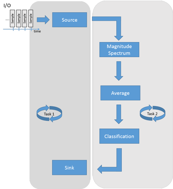
Threshold value monitoring of averaged magnitude spectra is to be implemented. The following components of the Condition Monitoring Library with the described functions are used:

• FB_CMA_Source
• Buffers of the input data
• FB_CMA_MagnitudeSpectrum
• Arrangement of the input buffers into overlapping sections
• Windowing of the calculation sections
• Calculation of the Fourier transformation
• Calculation of the absolute value of the Fourier coefficients
• Scaling of the result (RMS)
• FB_CMA_MomentCoefficients
• Formation of the arithmetic mean value
• FB_CMA_BufferConverting
• Adjustment of the buffer dimensions for transfer between FB_CMA_MomentCoefficients and FB_CMA_DiscreteClassification
• FB_CMA_DiscreteClassification
• Monitoring of each calculated frequency for threshold value violation

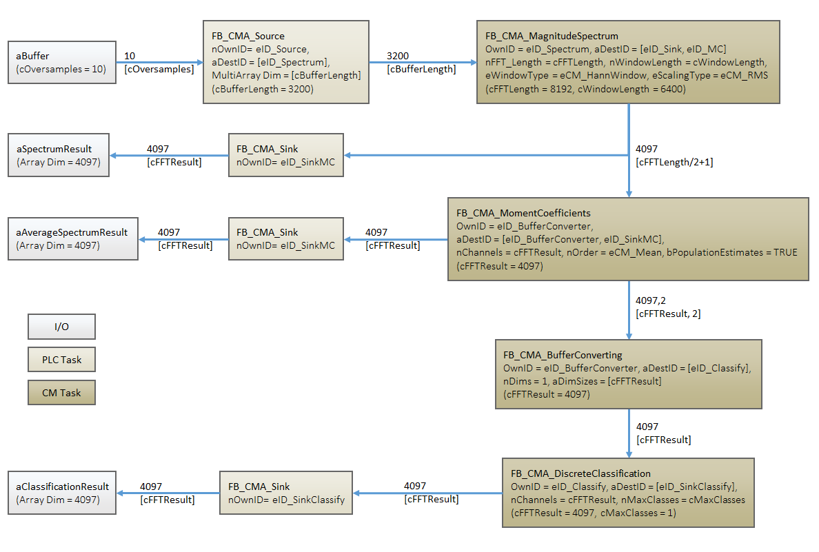
In a representation of the above diagram that is closer to the source code, a possible implementation is as follows:

The sample project for the concept shown here can be downloaded from here: Threshold value consideration for averaged magnitude spectra.

Parameterization of the calculation of a magnitude spectrum

The cycle time and the oversampling factor are set such that the resulting sampling rate is 10 kHz. The following settings are used in the sample for parameterization of the MagnitudeSpectrum function block and the source function block

// constant for input
cOversamples  : UDINT     := 10;    // number of oversamples
cFSample      : UDINT     := 10000; // 1ms task with 10 oversamples = 10kHz
    
// constants for FFT (Magnitude Spectrum)
cBufferLength : UDINT  := 3200;             // buffer size
cWindowLength : UDINT  := 2*cBufferLength;  // 50% overlap
cFFTLength    : UDINT  := 8192;             // length of FFT for mag. spectrum, power of 2
cFFTResult    : UDINT  := cFFTLength/2+1;   // result of mag. spectrum

The numerical frequency resolution is 10 kHz / 8192 = 1.22 Hz. As described in the context of zero padding and Frequency resolution, this does not correspond to the frequency resolution, which enables two adjacent frequencies to be distinguished. In this case this is 10 kHz / (2*3200) * 1.5 = 2.34 Hz; 2*3200 corresponds to the length of the signal section used for calculating the FFT (measuring time in sampling values). The expansion factor of 1.5 is defined through the choice of the Hann window (windowing in the MagnitudeSpectrum function block). The FFT-length of 8192 is the smallest number greater than 2*3200 representing a power of two. The length of the result array from the calculation of magnitude spectrum is 4097. It is defined through the symmetry property of the FFT.

Averaging of the magnitude spectra

The result of the MagnitudeSpectrum function block is transferred to FB_CMA_MomentCoefficients, which is configured such that it returns the average value (first central moment) as result. By default, the function block also provides the sample size that was used for calculating the central moment. For this reason the result array becomes two-dimensional. The present sample uses the CallEx() method of the function block to average 25 magnitude spectra and then reset the function block. Since in this case the sample size is always 25, this information is no longer required. The corresponding sink function block is therefore parameterized such that only the mean values are copied from the function block result to the context of the PLC task. In addition, a buffer conversion (FB_CMA_BufferConverting) is applied between the classification function block and the MomentCoefficients function block, which also omits the column containing the sample size information.

Classification

In the present case, the function block FB_CMA_DiscreteClassification is used as simple threshold value classifier. Accordingly, only two classes are defined (nMaxClasses = 1). The configuration of the threshold values, which is applied individually for each discrete frequency, takes place at runtime. In the sample the threshold value for array indices 30 to 50 (corresponding to approx. 36 Hz to 61 Hz) is set to 6 V_RMS, for the remaining frequencies it is set to 2 V_RMS. If the value falls below the threshold value, -1 is returned as result for the corresponding frequency. If the threshold value is exceeded, 0 is output.

Further information on the sample code

The project includes a measurement project, which contains a scope array project with three axes. The upper diagram shows the result of FB_CMA_MagnitudeSpectrum, i.e. the magnitude spectrum of the input signal. The input signal is generated by a function generator and represents a noisy sine wave with a frequency of 50 Hz and an amplitude of 25 V. Accordingly, the result of the non-averaged magnitude spectrum is time-variable (uncertain). Averaging stabilizes the result noticeably. The averaged magnitude spectrum is shown in the center of the Scope Array Project. The lower diagram shows the classification result; for each frequency -1 is shown if the value is below the threshold, 0 is shown if the defined threshold value is exceeded.

Further example for Condition Monitoring with frequency analysis

The Examples section contains several code examples. Section Condition Monitoring with frequency analysis contains an example that is similar to the one described in this section. It is intended to illustrate the flexibility your individual solution, which you can create with the Condition Monitoring Library.