Fourier analysis

Introduction

The most important frequency analysis method is the Fourier analysis. The fundamental significance of the Fourier analysis arises from the fact that it decomposes a signal x(t) into superimposed sine and cosine vibrations. The result of this transformation is referred to as signal spectrum or simply spectrum. Definition of the Fourier transformation:

In terms of information content, the signal spectrum is equivalent to the original signal. In addition, it provides information on the origin of vibrations, for example. If two machine components give rise to vibrations with different periods (frequencies) that are additively superposed, the Fourier transform makes these two components visible. The combination of sine and cosine for each frequency also enables phase angles to be mapped.

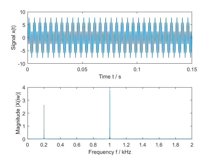
For example, superimposition of two sine waves with different frequencies and amplitudes results in the diagram shown below. From the variation over time it is difficult or impossible to glean the composition of the resulting signal. Conversely, from the magnitude spectrum |X(w)|, i.e. the magnitude of the Fourier-transformed, it is easy to see with appropriate scaling (see Scaling of spectra), that there are two oscillations – one with a frequency of 0.2 kHz and an amplitude of 2.6 and one with a frequency of 1 kHz and an amplitude of 3.8. The phase information is hidden due to the absolute value calculation.

In the Magnitude spectrum: sample, the magnitude spectrum is calculated and displayed for a signal of this form.

There are two processes that influence the vibration signals originating in a machine during sound transfer. Firstly transfer via machine components that attenuate the vibrations to different degrees depending on the frequency, and secondly superposition with vibrations from other machine components, with amplitudes adding up without interaction. Both factors are separated due to the properties of the Fourier transformation:

• Delays only affect the phase of the Fourier transform
• Frequency-selective attenuation and constructive superposition of vibration amplitudes show up in the magnitude of the Fourier transform.

Processing of time-discrete signals and the discrete Fourier transform

A very important aspect in the application of Fourier analysis is temporal sampling of the signal. The Fourier transform is mathematically defined for continuous, temporally unlimited signals.

However, in practice the discrete Fourier transformation (DFT) is used. It is defined for a discrete, periodic signal with a finite number of discrete frequency components. "Discrete" means that the signal is scanned at equal intervals, usually directly with an analog/digital converter, e.g. an EL3xxx or ELM3xxx.

If a time-continuous signal with a period of T is sampled, the resulting value string is:

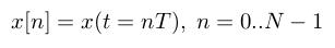
Using DFT, this series, which consists of N values, can be transformed to a discrete spectrum.

The variable k represents a frequency channel, which also referred to as frequency bin. Like the variable n, it runs from 0 to N ––1.

Discretization of time and quantization of values (digitization)

Two operations are required for digital processing of analog signals: Quantization from analog to digital value representation, and sampling of the temporally continuous physical signal to form a discrete sequence of quantized values.

The analog-to-digital converter digitizes the measured values in the I/O terminal. Quantization of the values generally takes the form of an integer signal with signed 16-bit representation or 24-bit representation. Processing in the TwinCAT 3 Condition Monitoring Library consistently takes place in the 64-bit IEEE double floating point format, which is hard-wired in advanced processors. The temporal sampling also takes place in the I/O terminal, through sampling of the input signal with a defined sampling frequency. The sampling frequency can be calculated from the task cycle time T_c and the oversampling factor c_s:

Sample: With a task cycle time of 1 ms and an oversampling factor of 10, the resulting sampling rate is f_s = 10 * 1 / ( 10^-3 * 1s ) = 10 kHz.

Pay particular attention to the sampling frequency In TwinCAT the sampling frequency results from the task cycle time and the oversampling factor of the terminal used: fs := Oversamples*1000.0/TaskCycleTime_ms. Caution: The unit milliseconds is used for the task cycle time, as usual in TwinCAT. The Task Cycle Time can be queried in the PLC via the global data type PlcTaskSystemInfo. See: INFOSYS Global Data Types

Sampling theorem

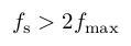
The main practical limitation in the application of the DFT is the restriction of uniquely representable frequencies. According to the Nyquist theorem or sampling theorem, only signals whose highest frequency f_max is less than half the sampling frequency f_s can be represented unambiguously (slightly simplified description). Accordingly, the sampling frequency must be greater than the highest frequency occurring in the analog signal.

The presence of higher frequencies in the analog signal leads to an undesirable effect referred to as aliasing in the spectrum. The analog signal is then no longer correctly represented in the discrete signal. Before the analog-to-digital conversion, higher frequencies should therefore be removed from the analog signal using configurable analog filters.

Anti-aliasing filter The EL3xxx and ELM3xxx EtherCAT Terminals provide various filters, depending on the terminal type. The EL3632 EtherCAT Terminal, for example, features a parameterizable analog 5th order low-pass filter, which is used to avoid aliasing. The EL3751 and the ELM3xxx modules have several filter levels that can be designed for anti-aliasing filtering as well as for wanted-signal filtering, see also TC3 Filter Designer.

Frequency resolution

Since the frequency resolution (discrete resolution based on frequency components in the signal) enables different signal components to be allocated to certain machine elements and defects, in many cases it will be of advantage to achieve a resolution of the discrete frequency axis that is as high as possible.

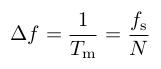
Generally, the length of the Fourier transformation N determines the step size Δf of the discrete frequency axis k ^.Δf. A basic consideration facilitates understanding: In order to be able to represent the frequency of a sine wave in the frequency range, the measuring time must be at least one full period of this vibration. This results in the following relationship between the resolution Δf and the measuring time T_m:

Typical PLC code syntax, e.g. in the MAIN routine of the Magnitude spectrum: sample:

fSampleRate := cOversamples * (1000.0 / fTaskCycleTime);

fResolution := fSampleRate / cFFTLength;

A high frequency resolution therefore requires a long measuring time. It is possible to extend the input data for the DFT through symmetric addition of zeros before and after the input signal (zero padding). This increases the length N of the signal sequence at constant sampling rate f_s, thereby refining the discrete resolution Δf. Zero padding does not add additional information to the signal. A distinction is made between two different types of resolution when zero padding is used: on the one hand the step size between one frequency bin to the next on the discrete frequency axis, i.e. the transition from k^.Δf to (k +1)^.Δf , on the other hand the resolution for distinguishing between two adjacent frequencies of the input signal.

Although zero padding reduces the discrete resolution Δf, it does not change the measuring resolution. A refinement of the measuring resolution can only be realized through a correspondingly long measuring time (often called WindowLength in the Condition Monitoring library for FFT-based algorithms). For practical applications, the key factor is usually the frequency resolution of the measurement, which influences the differentiability between two closely adjacent signal frequencies.

Zero padding Zero padding does not add any information to the signal to be analyzed. For distinguishing between two adjacent signal frequencies, it is therefore not the frequency resolution that is refined, only the numeric resolution of the frequency axis.

Illustration based on an example:

With a task cycle time T_c = 1 ms and an oversampling factor of 10 (i.e. f_s = 10 kHz), a buffer with a length of 3200 is filled. The resulting measuring time is T_m = T_c * 3200 / 10 = 320 ms, with a measuring resolution of Δf = 1 / 320 ms = 3.125 Hz. Using FFT for further analyses/calculations, the buffer is symmetrically expanded with 2*448 zeros to reach a length N of 2^12 = 4096 > 3200 (N must be a power of 2, see next section). Zero padding therefore refines the numerical resolution to Δf = 10 kHz / 4096 = 2,44140625 Hz.

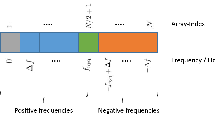
The discrete frequency axis is limited by the zero frequency (off-set) and the Nyquist frequency f_nyq, which corresponds to half the sampling frequency. According to the Nyquist theorem, it corresponds to the highest representable frequency of the recorded signal. If the discrete spectrum X[k] is saved in a PLC array with the index m, which runs from 1.. N, the following frequency axis results for X[k]

fFrequency := (m-1) * fResolution; // m = 1..N/2+1

m = 1 represents the off-set, m = N/2+1 represents the Nyquist frequency. The indices for m from N/2+2 to N form the so-called negative frequencies, which are only relevant in practice if the input signal x[n] for the FFT has a complex value. See section Fourier analysis.

The following diagram illustrates the configuration of the frequency axis for a DFT of length N (with N an even number).

Efficient calculation through FFT algorithms

Strictly speaking, the fast Fourier transformation (FFT) is a family of algorithms for discrete Fourier transformation (DFT) which are implemented particularly efficiently and lead to the same numerical result. While the complexity of a naïvely implemented DFT with N time values is O(N ²), for a FFT it is only O (N * logN). For larger values of N, the difference is substantial. For N=1024, for example, it is already a factor of around one hundred. Generally FFT algorithms are defined for values of N (the length of the FFT) that represent a power of two, i.e. 256, 512, 1024 etc.

Complex valued result

The FFT (and the DFT) splits the incoming signal x[n] into a number of sine and cosine oscillations. Each frequency is associated with a coefficient for the sine and cosine components. Both factors are represented together as a complex number. The decomposition is expressed in Euler's formula:

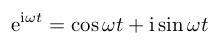
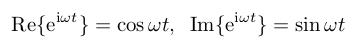
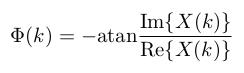
The real part Re{..} of each Fourier coefficient corresponds to the cosine component, the imaginary part Im{..} to the sine component. The ratio of the two components reflects the phase angle of the frequency components.

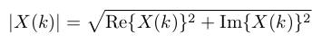
In many cases it is not the precise temporal characteristic of the signal that is of interest, but the magnitude spectrum. This can be determined from the Fourier transform by calculating the absolute value of the complex number:

Complex data type The result of the FFT of a real-valued or complex-valued input signal is complex-valued. The data types LREAL and LCOMPLEX are used for the signal representation. If a function block is used for calculating the FB_CMA_MagnitudeSpectrum or FB_CMA_PowerSpectrum, the result is directly real-valued.

Image frequencies

In the Fourier transform of a real signal the coefficients for negative frequencies are equal to the complex conjugate coefficients for positive frequencies. If X[k] is the Fourier-transform of x[n] and X*[k] the complex conjugated, the following applies for a Fourier transformation with N points:

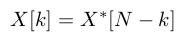
For real-valued signals a time reversal of the input signal corresponds to complex conjugation of the Fourier transform. It follows that the spectral value for frequencies below the Nyquist frequency occur mirrored in the values above the Nyquist frequency. Since the values with k > N/2 are therefore redundant for real input sequences, the Fourier-transformed for real sequences is usually limited to the first n/2 values (applies to k = 0..N––1).

Overview of the calculation of spectral values

The Condition Monitoring library offers a variety of ways to calculate spectral values. The following table offers an overview. The relationships of the FFT with (overlapping) windows will be considered in detail in the next chapter.

Here, N corresponds to the FFT length, L to the window length (or overlapping respectively) and nBins to the number of configured spectral values. Furthermore, D designates the decimation factor. The length of the input data buffer of the function block FB_CMA_SlidingDFT is not restricted to a fixed size. The lengths L, V of the order spectrum must be specifically adapted to vibration and position data.