Scaling of spectra
Magnitude and power spectrum
There are several common ways of evaluating the spectrum:
- The FB_CMA_MagnitudeSpectrum, which uses linearly scaled magnitude values of the complex-valued spectral values |X[k]|. It is also called the amount spectrum or amplitude spectrum.
- The FB_CMA_PowerSpectrum, whose values represent the squares of the magnitude values |X[k]|2.
Using the power spectrum makes sense if power values are added up or consolidated, since the squared spectral values |X[k]|2 relate exactly to the RMS value of the time signal via Parseval's theorem.
According to Parseval’s theorem, the power of signal x[n] in the time representation equals the power of the signal in the Fourier transform:
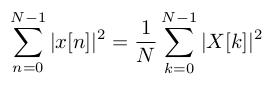
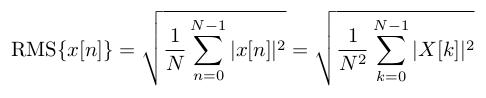
If one now calculates the RMS value of the signal x[n], this can be realized in the time range or in the frequency range, since both representations are identical with regard to the power:
In practice this allows RMS values, for example, to be calculated for limited frequency ranges of a signal. Practical Spectrum Scaling Options of the Condition Monitoring Library, which relate to the properties referred to in this section, include eCM_ROOT_POWER_SUM and eCM_RMS.
The power spectral density
Another important concept for spectral analysis is the Power Spectral Density (PSD). It refers to the output value based on the effective frequency resolution, as indicated by the Equivalent Noise Bandwidth (ENBW)
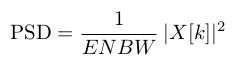
A look at the physical units for the signal, magnitude spectrum and PSD illustrates the relationships. If a signal x[n] is measured in volt (V), the discrete magnitude spectrum |X[k]| is also stated in V. Squaring means that the power spectrum is stated in V2. By definition, the power density spectrum is a power value (V2) based on the frequency in Hz. Relating the power spectrum to the effective frequency resolution in hertz (Hz) results in the unit V2/Hz.
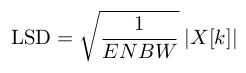
This representation can also be used for magnitude values. Correspondingly, the linear spectral density (LSD) is
Decibel scale
The conversion of values from the linear to the logarithmic "decibel scale" is common in vibration analysis and machine acoustics. The decibel scale allows a good interpretation if both very large values and very small values occur in a spectrum and are to be evaluated in areas of both large and small values. The magnitude spectrum is converted to the decibel scale via:
The decibel scale can be calculated both over 10 times the logarithm of the power spectrum and 20 times the logarithm of the magnitude spectrum. The result of a calculation from FB_CMA_MagnitudeSpectrum and FB_CMA_PowerSpectrum is therefore identical in the decibel scale.
The conversion of results to the decibel scale is conveniently activated by the Condition Monitoring Library via a Boolean variable in the function block initialization parameters, see e.g. ST_CM_PowerSpectrum_InitPars.
Scaling options according to signal type
By selecting a suitable Spectrum Scaling Options, the spectral values calculated by the FB_CMA_PowerSpectrum or FB_CMA_MagnitudeSpectrum function block can be automatically adjusted to a desired reference variable. The correct interpretation of the reference variable is of particular importance here.
In practice, and assuming a stationary signal, it is important first of all with scaling options to distinguish between deterministic and stochastic signals.
Deterministic signals consist of periodic vibrations with a defined frequency. Decisive here is that the frequency resolution (ENBW) is wider than a harmonic frequency. Thus, the entire power of this frequency component of the signal is consolidated in this frequency channel. Therefore, the spectral values are directly scalable to an amplitude (Spectrum Scaling Options eCM_PeakAmplitude) or an RMS value of an equivalent sinusoidal signal. If the signal does not fall in the center of the frequency channel, so-called scalloping losses occur, compare section Window functions, which reduce the observed maximum amplitude. Apart from the use of a flat-top window, this can be compensated retroactively by the use of a Hann window, for example, in which the power values from neighboring frequency channels are evaluated as a sum, see Spectrum Scaling Options eCM_ROOT_POWER_SUM and eCM_RMS.
Stochastic or broadband signals necessitate the evaluation of Power Spectral Densities (PSD) or Linear Spectral Densities (LSD), since all frequencies contain signal power over a defined frequency range. In this case the determined power values depend on the effective width of the frequency channels of the FFT. Logically, they must be referenced to this bandwidth in order to obtain results that are independent of the evaluation parameters. Because the effective width of the frequency channels when using window functions depends on the length and shape of the window function, the above-mentioned Equivalent Noise Bandwidth (ENBW) must be used in this case, see Spectrum Scaling Options eCM_PowerSpectralDensity.
Scaling on the basis of the PSD does not enable consistent scaling of the "DC component". If required this should be determined by low-pass filtering or averaging.
If a signal contains both deterministic portions and wide-band portions, both scalings must be used independently of each other in order to obtain values that are independent of the processing parameters. One example would be the evaluation of a signal that is composed of a harmonic sine wave and band-limited noise. If the amplitude of the harmonic sine wave is to be evaluated, then scaling for deterministic signals must be carried out. If one strives to assess the stochastic background noise, then scaling must be carried out as PSD or LSD.
 | Scaling of spectra with the Condition Monitoring library Various scaling options are already implemented in the Condition Monitoring library and can be parameterized via the function-block-specific structure with initialization parameters. See E_CM_ScalingType and Spectrum Scaling Options. A tutorial on this can be found here: Scaling of spectra. |
Referencing
Classification of the scaling
While comparison of absolute measured values is very important for measurement technology, for vibration assessment according to ISO 10816-3 and for machine protection, absolute calibration is not required for trend-based or comparative condition monitoring.
In many cases, generic limit values that are not tailored to a specific machine, are less suitable for early diagnostic detection of damage. Since the choice of measuring point (location of the measurement, coupling of the sensor etc.) has significant influence on the attenuation factors of the transmission link, for trend monitoring it is much more important to consistently maintain the selected test point and the coupling conditions. In many cases signal components with initially low signal level can be important. If they are periodic, they appear particularly clearly and early when using high-resolution FFT spectra with the narrowest possible bandwidth and suitable statistical functions. In condition monitoring trend observations over long periods and relative comparisons at the decibel scale usually play a much more important role than individual absolute values. For the sensors this means that expensive, high-precision absolute calibration and smooth frequency response are generally less important than high long-term stability and sufficiently low temperature dependence, although this does not mean that a calibration can be neglected completely.
Scaling on the basis of reference signals
In many cases, mathematical referencing (scaling by means of a reference) of measured values be much more complex than would appear at first glance. As soon as the processing involves several steps that are non-linearly dependent on diverse parameters, it is in many cases simpler and above all less prone to error to carry out the scaling with the aid of a calibration device. Here we make use of the fact that the magnitude values of the calculated spectra are always linear to the input values. In order to scale the signal correctly, therefore, we only need to determine the associated linear factor on the basis of a well-known reference input value. Professionally this is done by generating a physical signal with a defined amplitude (or a defined RMS value) using a calibration device, measuring the output value and determining the required correction factor as the quotient of input and output. The big advantage of scaling on the basis of a reference signals is that physical defects such as damage to an accelerometer as well as incorrect configurations of the measuring system can be reliably discovered. This method has its limits if a large number of parameter combinations are to be tested when evaluating.