Statistical analysis

Basic concepts

If a quantity (e.g. temperature, pressure, voltage etc.) is measured in an actual process, for a repeated measurement it is very likely that the previous measured value does not match the value determined in the repeat measurement. Since the sequence of randomly fluctuating quantities cannot be determined deterministic (i.e. via a concrete equation), statistical parameters are used for describing such signals. The fact that in practice deterministic and stochastic signals are often superimposed (e.g. a direct voltage superimposed by measurement noise) is irrelevant. The summary result is random and therefore a stochastic signal.

An individual measurement of a randomly fluctuating quantity is a random event. Each individual measurement is referred to as realization of a random experiment. If N random samples are taken from the random experiment, this number of realizations describes the sample size.

Histograms

A central property of random events is the probability that the measured parameter assumes a certain value. This is described via the absolute or relative frequency distribution, which is represented in a histogram.

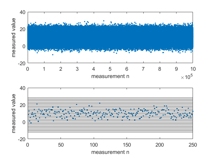
Simple example: Suppose a measured variable of 10 V is superimposed with normal distribution noise (average value 0 V, standard deviation 4 V). Repeating the measurement for this parameter 1 million times results in the diagram below (upper part). The 1 million realization of the random experiment can be shown in a histogram for a better overview. The absolute frequency distribution can be generated such that the range of the measured variable is subdivided into classes (bins). The upper part of the diagram shows the measured variable over each individual measurement, the lower part only shows the first 250 measurements and the class limits for the histogram.

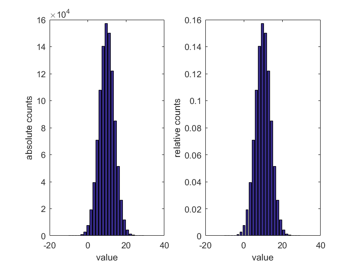
The absolute frequency distribution is then simply results from the number of measured values that lie within a class (bin), see diagram below, left. The distribution is parameterized based on the number of considered classes – the more classes, the finer the distribution. The relative frequency distribution can be calculated from the absolute frequency distribution through referencing of the sample size; see diagram below, right. This is then independent of the number of measurements and shows the probability with which a value was measured, e.g. values in the class around 10 V were measured with a probability of 0.157=15.7%.

An experimentally investigated process can initially be visually assessed quite easily on the basis of a frequency distribution. Three questions can be explored:

• How strong is the scattering of the measured value?
• Is the measured value scattered around a single value (as above around 10 V), or around further values?
• How are the values distributed? - normal distribution, Student's t-distribution, chi-square distribution?

Calculation of absolute frequency distribution in TwinCAT 3 The Condition Monitoring Library can be used to calculate the absolute frequency distribution conveniently via the function block FB_CMA_HistArray. Only the range under consideration and the number of classes are required for parameterizing the function block. A graphic display is possible with the array bar chart in TwinCAT Scope View. A sample is available for download from Histogram. The Statistical methods sample illustrates further Condition Monitoring Library options for statistical data evaluation.

Ordinary and central moments

A value that is as close as possible to the actual value can be estimated based on multiple observations of a random process. It is referred to as best estimate. Different estimators (e.g. the arithmetic mean) with different properties can be used for this purpose. In addition to the calculation of the best estimate, in many cases it is important to also express the uncertainty of the estimate, which is usually calculated via the experimental standard deviation (also referred to as empirical standard deviation).

For example, the moments are very well suited for calculating statistical variables from a given sample: average value, variance, skew, kurtosis etc. are particularly suitable for calculating statistical parameters from a given number of operations. While the average value provides a suitable estimate, the other moments provide insight into the distribution of the values around this estimated value.

Illustration based on a sample:

The sample described above under histogram has a "true value" of 10 V and was retrospectively subjected to noise. From the given sample of 1 million realization the average value can be calculated as 9.9977 V. This is the best estimate of the true value. The variance around this average value is 16.01 V². The root of the variance corresponds to the standard deviation and is 4.0013 V. If the distribution of the measured values is normally distributed as in this case, then the distribution of the measured values is completely described with these two moments, i.e. the skew and kurtosis are (theoretically) zero. The skew describes the symmetry of the distribution around the average value, the kurtosis describes the steepness (peakiness) of a distribution function.

Assessing the uncertainty of an estimated result:

In 1995 the Joint Committee for Guides in Metrology (JCGM) published a guide on stating measurement uncertainty. The JCGM is composed of central umbrella organizations such as BIPM, IEC; IFC, ISO etc., who developed this guide as a joint effort. The basic paper "Guide to the Expression of Uncertainty in Measurement" (GUM) is available for download free of charge from the BIPM website. A brief introduction into the central idea is provided below.

As described above, a best estimate can be calculated from a given set of N observations (average value = sample mean). The variance of the best estimate is calculated and used as uncertainty value, rather than the variance of the set of observations (standard deviation). This makes sense, because the aim is to assess the uncertainty of the estimated value. The variance of the best estimate can simply be calculated from the standard deviation of the set of observations by dividing this value by the root of N. If the sample size is sufficiently large, the uncertainty value can be multiplied by 2 (otherwise a larger factor), in order to calculated the extended uncertainty. The average value plus/minus this extended uncertainty will then contain the true measured value with a probability of 95%.

Accordingly, the algorithms of the Condition Monitoring Library can be used to make GUM-compliant statements on the measurement uncertainty.

Calculation of moments in TwinCAT 3 With the Condition Monitoring library, the function block FB_CMA_MomentCoefficients can be used to calculate the first to fourth order moments (mean, variance, skew, kurtosis) of a sample. The function block only has to be parameterized in terms of the sample size used.

Quantile

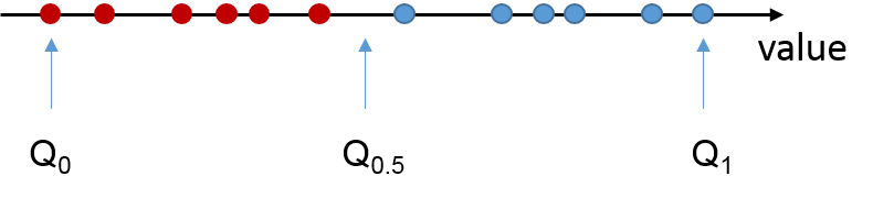
The p-quantile Q_p of a random variable x is the value for which Q_p is greater than x for the portion p of all realizations of x. A little more descriptively formulated: If a finite number of values is given, then the p-quantile divides the data into two areas. The 50%-quantile (median), for example, marks the value below which at least 50% of all the values lie. This value should not be confused with the mean of a sample.

The value of p can lie between zero and one. If p is specified in percent, then percentiles are concerned. Q_0.5 thus corresponds exactly to the median, while Q_0.9 is the 90% percentile and Q₁ is the maximum of an observed sequence of values.

The closer p approaches the value of one, the more Q_p is determined by outliers and extreme individual values, and the closer p approaches the value of 0.5, the more Q_p approaches the median, which is very robust against outliers. The value of p, which can be configured in TwinCAT at runtime, can be used to dynamically change the sensitivity of the evaluation of a sample to individual values.

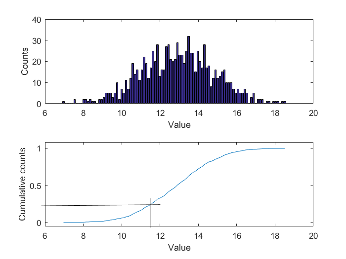
To illustrate the basic idea of quantiles, the following graphic shows a sequence of 1000 values scattered around a mean value of 13.

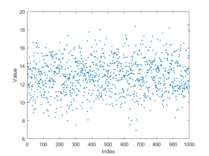
From the value sequence, a histogram can be calculated that indicates how often a value occurs in the sequence under consideration (sample). By integrating the absolute frequency shown in the histogram and referencing to the total number of values in the sequence under consideration (in this case 1000), the empirical sum frequency distribution can be calculated, on the basis of which the quantiles can easily be read. In this case, for example, the 25% quantile is 11.8, i.e. at least 25% of the individual values of the sample of 1000 values under consideration lie below this value.

The library function block for calculating FB_CMA_Quantiles works in two sub-steps, which can be called together or in separate sub-steps. In the first step values are added to an internal histogram, whose parameters can be configured in advance. This step requires very little computational effort. In the second step, the previously selected quantiles are calculated from the stored histogram. Depending on the configuration this second operation is computationally much more intensive, because it is defined by more complex operations, but it needs to be performed much less frequently.

Calculation of quantiles in TwinCAT 3 The function block FB_CMA_Quantiles can be used for the calculation of quantiles. Several quantiles can be calculated with just one function block call. The function block is parameterized like the histogram function block, as well as the quantiles to be calculated and the sample size to be used.