Configuration structures
General description
An individual configuration structure ST_FTR_<type> exists for each function block FB_FTR_<type>. In the configuration structure all parameters are defined that are required for the calculation of the transfer function, the input and output variables (size and form of the arrays) as well as the internal states.
Common parameters
All configuration structures ST_FTR_<type> contain the following parameters:
Parameter | Type | Description |
|---|---|---|
| UDINT | Number of oversamples > 0 |
| UDINT | Number of channels > 0 & < 101 |
| POINTER TO LREAL | Pointer to array with initial values (optional) |
| UDINT | Size of the array with initial values in BYTE (optional) |
nOversamples and nChannels
The parameters nOversamples and nChannels describe the size of the input and output arrays that are transferred when the Call() method is called. If, for example, 10 oversamples and 3 channels are used, the Call() method expects an array with 30 elements at the input and output (see Oversampling and channels).
The parameter nChannels describes the number of parallel signal channels to be processed with a call. The parameter nOversamples describes the number of samples that occur for each individual channel and each call of the Call() method.
Inital Values
The optional parameters pInitialValues and nInitialValuesSize are used to define the internal state of the filter after its configuration. In practice, the parameters are used to reduce the settling time of the configured filter by introducing prior knowledge. For this purpose, the historical values y[n-k] and x[n-k] with k > 0 in the difference equation must be set in a targeted manner.
The following structure of the difference equation applies to the function blocks FB_FTR_IIRCoeff, FB_FTR_MovAvg, FB_FTR_PT1, FB_FTR_PT2 and FB_FTR_PT3:
|
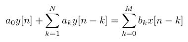
For a more compact illustration, the following notations are used for the historical values: xi,k and yi,k, where channel i and time delay k > 0. Sample: Channel i = 2 and delay k = 3 corresponds to y2,3 = y2[n-3].
Application options:
InitialValues = nullptrAll historical values yi,k and xi,k with k > 0 are set to zero for all channels i. This corresponds to the behavior if the entries of the structure are not used.InitialValues = PAll historical values xi,k, where k > 0, are set for all channels i to the value P. All historical values yi,k with k > 0 are set to V*P for all channels i, where V corresponds to the DC gain of the filter.
Accordingly, the filter is in steady state for all channels with respect to a constant input signal x[n] = P.InitialValues = [x1,1,x1,2,…,x1,M,y1,1,y1,2,…,y1,N]All historical values xi,k with k > 0 and yi,k with k > 0 are set individually, but to the same values for all channels i.InitialValues = [x1,1,x1,2,…,x1,M,y1,1,y1,k,…,y1,N ,
x2,1,x2,2,…,x2,M,y2,1,y2,2,…,y2,N ,
…….
xI,1,xI,2,…,xI,M,yI,1,yI,2,…,yI,N]All historical values xi,k and yi,k are set individually for every channel i = 1..I.
For the function blocks FB_FTR_IIRSos and FB_FTR_IIRSpec, the transfer function is calculated in second-order sections (SOS):
|
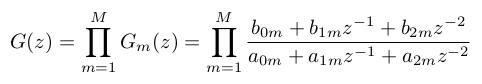
The compact illustration is extended accordingly by m, which specifies the biquad: x(m)i,k and y(m)i,k. Sample: Channel i = 2 and delay k = 1 of the fourth biquad (m = 4) corresponds to
y(4)2,1 = y(4)2[n-1]. Each biquad can use only two historical values here; accordingly, k = 1.2.
Therefore, the structuring for the input and output values is different there.
Application options:
InitialValues = nullptrSame behavior as described above.InitialValues = PSame behavior as described above.InitialValues = [x(1)1,1,x(1)1,2,x(2)1,1,x(2)1,2,…,x(M)1,1,x(M)1,2,
y(1)1,1,y(1)1,2,y(2)1,1,y(2)1,2,…,y(M)1,1,y(M)1,2]All historical values x(m)i,k and y(m)i,k are individually set, but the same for all channels i.InitialValues = [x(1)1,1,x(1)1,2,x(2)1,1,x(2)1,2,…,x(M)1,1,x(M)1,2,
y(1)1,1,y(1)1,2,y(2)1,1,y(2)1,2,…,y(M)1,1,y(M)1,2,
x(1)2,1,x(1)2,2,x(2)2,1,x(2)2,2,…,x(M)2,1,x(M)2,2,
y(1)2,1,y(1)2,2,y(2)2,1,y(2)2,2,…,y(M)2,1,y(M)2,2,
…….
x(1)I,1,x(1)I,2,x(2)I,1,x(2)I,2,…,x(M)I,1,x(M)I,2,
y(1)I,1,y(1)I,2,y(2)I,1,y(2)I,2,…,y(M)I,1,y(M)I,2]
All historical values x(m)i,k and y(m)i,k are set individually for every channel i = 1..I.
The function block FB_FTR_PTn is also described as a cascaded filter, but as a first-order cascaded filter. Accordingly, the same consideration as for the SOS blocks applies here, but with k = 1. For a PTn filter where n = M, the following then applies:
InitialValues = nullptrSame behavior as described above.InitialValues = PSame behavior as described above.InitialValues = [x(1)1,1,x(2)1,1,…,x(M)1,1,
y(1)1,1,y(2)1,1,…,y(M)1,1]All historical values x(m)i,k and y(m)i,k are individually set, but the same for all channels i.InitialValues = [x(1)1,1,x(2)1,1,…,x(M)1,1,
y(1)1,1,y(2)1,1,…,y(M)1,1,
x(1)2,1,x(2)2,1,…,x(M)2,1,
y(1)2,1,y(2)2,1,…,y(M)2,1,…….
x(1)I,1,x(2)I,1,…,x(M)I,1,
y(1)I,1,y(2)I,1,…,y(M)I,1]
All historical values x(m)i,k and y(m)i,k are set individually for every channel i = 1..I.