Bearing monitoring

Motivation

Bearings are among the commonest and most highly stressed machine elements. In many cases they can be of critical importance for the operation of a plant. While the downtime alone can cause high costs for the procurement of spare parts for large bearings, the failure of small bearings can also cause costs that far exceed the costs of the spare part.

Causes of damage

There are many different possible causes of the failure of roller bearings:

• The ‘natural’ cause of the failure of roller bearings is material fatigue due to the high stresses that occur on the contact surfaces of the rolling elements during operation. After a certain time these lead to cracks in the material and to break-outs on the running surface. Small defects result that initially grow very slowly and become larger with increasing speed towards the end of the fatigue life. The mechanisms of material fatigue are understood well in theory and can be statistically described; they are a component of normal wear. In designing a normal bearing the dimensions are selected such that the probability of serious damage within the fatigue life of the machine is low. Under normal circumstances, therefore, it can be expected that correctly dimensioned and maintained bearings will have a very long fatigue life. The fatigue life actually attained is often considerably shorter, but not accurately predictable and can vary considerably due to the following causes.
• The stress on rolling elements and running surfaces is significantly increased by incorrect lubrication, since the lubricant distributes part of the stress and also prevents the bearing from overheating.
• A further cause of damage is contamination, for example due to faulty seals or metal swarf. The penetration of water can also lead to the failure of the lubrication, since even small amounts of water render lubricants unusable.
• Further, not unimportant sources of error are inaccuracies in the alignment or damaging stresses during the installation.
• Excessive stresses lead to plastic deformations of the running surface (brinelling). A similar situation can be caused by vibrations when the bearing is at a standstill, which are not mitigated by a lubricant film (false brinelling).
• In electrical machines the flow of current can destroy the running surfaces.
• Corrosion can be the cause of the initial surface damage.

The common factor in all these causes is that damage to the contact surfaces of the roller bearing can be detected at an early stage. From the fact that, in the overwhelming majority of cases, bearing failures are not caused by material fatigue, it follows that the early recognition of damage and the analysis and tracing of the primary causes (Root Cause Failure Analysis (RCFA)) make it possible in the mid-term to preventively avoid many types of damage and to significantly prolong the service lives of bearings, in addition to reducing downtime costs.

Consequences of damage

Following the initial damage to the running surfaces, the increasing stresses result in the spreading of defects. Apart from the running surface other components can also be affected, such as the cage of the rolling elements. Vibrations do not necessarily indicate the first stages of the damage process, since they usually represent a symptom rather than a cause of the damage. Nevertheless, all damage processes lead sooner or later to defects at the points of contact, which express themselves in the form of increasing vibrations.

Monitoring strategies

Since the direct recognition of the first causes may be difficult, the focus is placed on the early recognition of the consequential damage to the running surface of the bearing. The earlier this is noticed and investigated, the greater the chances are of finding the initial damage and rectifying it on the basis of the causes. This strategy often leads to sustainable savings in the long run. Furthermore, early recognition facilitates the planning of maintenance, which is an advantage above all for plant operators. Another strategy is to identify the elements concerned by analyzing the vibration signals.

To aid understanding of the following signal analysis options, a short phenomenological introduction into the formation of vibrations in defective roller bearings is provided.

Schematic cross-section of a roller bearing:

The critical parts of a roller bearing are moving surfaces in contact with each other. These are the rolling element surface, the contact surface of the inner race and the contact surface of the outer race. Rolling over local damage in a contact surface results in a shock pulse, which can be picked up by an accelerometer. The more severe the damage, the stronger the shock pulse.

The crest factor

The crest factor is defined as the ratio between the maximum amplitude and the RMS value of the signal. It is specified in decibel and is a number greater than or equal to zero. The crest factor thus determines the relationship between maximum amplitude and the effective mean measured oscillation amplitude. Shock pulses resulting from incipient damage lead to an increase in the crest factor. The following diagram shows the increase in crest factor with increasing pulse content of the signals.

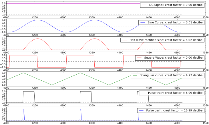
The bottom diagram shows the typical strong increase in the crest factor when acute shock pulses are encountered. An increase in the crest factor is usually a good indicator for damage. That makes this variable a suitable tool for the early recognition of damage and for trend analyses.

Signals from a roller bearing can be interpreted as follows.

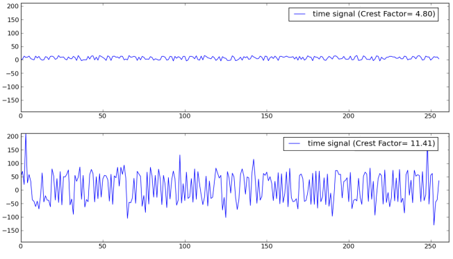
The diagram above shows two vibration signals from bearings with different wear, in each case with the corresponding crest factor. The signal sequence at the bottom clearly shows peaks resulting from damage. While the undamaged bearing has a crest factor of 4.8 dB, the damaged component has a value of 11.4 dB, clearly indicating the presence of damage.

The crest factor has the advantage that it is very efficient to calculate and easy to interpret. In addition, it can easily be displayed in a diagram over the time. In order to be able to use it correctly, it is important to understand the fundamental limits of this type of evaluation:

• The crest factor is strongly influenced by the signal maximum and is therefore not a robust parameter in a statistical sense.
• The crest factor increases with increasing local damage. However, above a certain degree of damage, the peak values of the shock pulses will no longer increase significantly, although the number of local defects will increase. As a result, the signal maxima will not increase, while the RMS value of the signal continues to increase. Consequently, for heavily damaged bearings the crest factor will fall again.

For this reason it is advisable to measure the crest factor continuously and analyze the results in terms of the trend.

The kurtosis value

In some cases the limited statistical robustness of the crest factor can be problematic. A more robust, yet somewhat more computationally demanding parameter is the kurtosis value (also referred to as curvature, fourth central moment). Like the average value and the variance, the kurtosis is a so-called moment coefficient, with can be used to describe parameters statistically. The kurtosis describes the ratio between the extreme values (far away from the mean value) of a distribution and the mean variation. Since occasional outliers in a measurement series have no significant effect on the result, the kurtosis is statistically much more robust than the crest factor.

In practice, the kurtosis tends to be used similar to the crest factor. The kurtosis (or the excess) and other common statistical moment coefficients are calculated in the TwinCAT 3 Condition Monitoring Library using the MomentCoefficients function block.

Processing concepts

The above diagram shows the function blocks available for calculating the crest factor and kurtosis. The FB_CMA_CrestFactor function block can evaluate data from several sensors at the same time, provided that the number of individual values is the same for each channel. The return value consists of an individual value for each channel. The individual values are returned in a vector. In the above diagram this is indicated by the arrows in horizontal and vertical direction. The crest factor function block in each case contains 5 individual values (vertical) for 7 channels (horizontal) and returns the crest factor for each of the 7 channels.

The kurtosis can be evaluated with the FB_CMA_MomentCoefficients function block. Here the values are transferred alternatively for all channels and individual time steps, or block-by-block for several time steps, which is more efficient for single-channel signals due to the smaller overhead.

Theory

The determination of the crest factor or kurtosis provides early pointers to the presence of damage with very little expenditure. Since the dismantling and inspection of components always entails expense – in some cases considerable – and in view of the fact that there may be a large number of bearings, additional diagnostic possibilities are of interest with which damaged bearings or even individual components can be more accurately identified. The identification of defects is based on the evaluation of shocks which can be traced back to damage to the contact surfaces. In case of damage to a rotating part, the shock pulses occur periodically, wherein the length of the period depends on the frequency with which a defect touches the contact surface. This shock pulse period depends on the speed of rotation of the bearing on the one hand and on the geometry of the element on the other. Hence, the period of the shock pulses can identify the defective component.

The shock pulses contain a high-frequency signal component, which is due to the vibrations of the activated machine component, and a superimposed (folded) and possibly also a modulated low-frequency component, which contains information about the periodic repetitions of the shocks. These low-frequency portions of the signal can be determined by the calculation of the envelope. The envelope can be calculated efficiently by applying the Hilbert transformation in the frequency range. Prior filtering by a high-pass filter, such as that provided by the TwinCAT 3 Controller Toolbox, may be useful, but is not absolutely necessary. Following the calculation of the envelope the power spectrum of the envelope signal is determined. The distinctive frequencies of this envelope spectrum identify the shock periods.

Application

The envelope spectrum is helpful in particular for diagnosing which units or which components of a bearing may be defective. In addition to that, the possibility of evaluating specific important portions of the signal and excluding interfering parts is of interest for the early recognition of damage. If they are to be used for early recognition, then the damage frequencies in question must be determined from the bearing geometry and monitored.

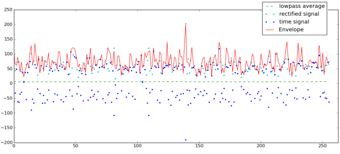
The above diagram shows the envelope of the signal of a damaged roller bearing already used before. The time signal is marked by the blue points, the envelope by the red line. For better understanding a green dotted line plots the sliding mean value of the time signal, which is not exactly zero, and the light blue line plots the amounts of the negative values in the time signal. It can be seen that the envelope always lies very close to the maximum values of the time signal or the amount of the time values. Peaks or negative deflections in the time signal lead to peaks in the envelope, whilst ‘background noise’ in the time signal is changed very little by the envelope formation.

Analysis of the envelope spectrum

Since a sequence of periodic shocks (pulse train) corresponds to a signal with many harmonics, the envelope spectrum contains the base frequency on the one hand and the integer multiples of the base frequency on the other. Just like for a power or magnitude spectrum, the frequency associated with the spectral values is derived from the index of the result array multiplied with the frequency resolution of the FFT; see Frequency resolution. with the length of the FFT N and the sampling rate f_s it follows: Δf = f_s ⁄ N and therefore for the frequency of the frequency bin with index m : f_m = (m-1) Δf (assuming the array index m starts with 1).

For diagnosis the base frequency of the pulse train must be identified. The harmonics are recognizable by a comb-like sequence of sharp maxima with an even spacing. The base frequency is the distance between these maxima, i.e. usually the frequency of the first maximum of this series. Their inverse value results in the period of the shocks; the unit of the inverse value is thus a time difference. Together with the rotational speed of the axis, which has to be measured, and the speed ratios of the damage frequencies, which can be determined from the bearing geometry, components from which the damage may have originated can be determined.

Characteristic damage frequencies in roller bearings

The illustration below shows by way of example the speed ratios that can occur in a simple roller bearing. In principle, shock pulses occur at the frequency with which the point of contact between two bearing elements passes a point with a damaged surface (on the upper side of the rolling element at the very bottom in the picture). This point of contact also moves due to the movement of the elements relative to each other. The rotary speed or angular speed of the point of contact can be determined based on the rule that there is hardly any slip in a correctly functioning bearing, which means that the elements roll off one another almost completely.

Roller bearing geometry parameter

Assume that the speed f_red of an axle connected to the inner ring is measured and the diameters of the bearing parts are as follows: Diameter of the inner race D_I, diameter of the balls D_B, diameter of the outer race D_A. The number of balls is Z. D_I and D_A give rise to the pitch diameter: D_P = (D_I + D_A)/2. Now if the inner race rotates with a speed of f_rot, then the pulse frequencies can be determined from this. The following acronyms are common for the designation of the frequencies:

• BPFO: Rolling element pass frequency outer race.
• BPFI: Rolling element pass frequency inner race.
• BSF: Bearing spin frequency rolling elements.
• BPF: Ball pass frequency.
• FTF: Fundamental Train frequency.

Contact angle:

For an accurate calculation in the case of bearings that bear axial loads, the diameter of the balls is to be corrected with the contact angle α with which the balls touch the running surface: D_b = cos(α) D_B. For radial bearings, this angle is 0°, which results in the following formulas used in practice:

BPFO = Z * f_red /2 * (1 - D_b / D_P)
BPFI = Z * f_red /2 * (1 + D_b / D_P)
BSF = f_red /2 * D_P/D_B * (1 - (D_b/D_P)²)
BPF = 2 * BSF
Rotating inner race:
FTF = f_red /2 * (1 - D_b/D_P)
Rotating outer race:
FTF = f_red /2 * (1 + D_b/D_P) Where (BPFI + BPFO) / f_red is always equal to the number of rolling elements Z. There are slight deviations from these formulas in practice, as the contact angle α can vary under load, for example. As a simple rule of thumb, the value

f_BPFI = 0.6 * f_red * Z

is used as an indicator frequency for a defect of the inner race, and

f_BPFO = 0.4 * f_red * Z

for a defect in the outer race. For the determination of the bearing geometry it is useful to refer to the bearing manufacturer’s data. It can also be helpful to use calculation programs, some of which the manufacturers offer on the Internet.

The type number of a roller bearing does not allow any clear conclusion to be drawn with regard to the bearing geometry; parameters such as the number of rolling elements can by all means change.

Processing concept

Frequency analysis processing steps

Analysis steps: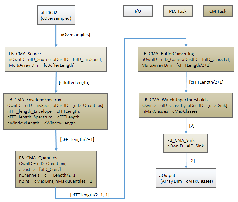

The above diagram shows the processing steps for the envelope spectrum as well as the function blocks that can be used here. First of all the envelope is calculated using the Envelope function block. Subsequently the power spectrum is calculated (PowerSpectrum) function block, in the same way as the spectrum for any time signal. Since the envelope spectrum obtained fluctuates relatively strongly with non-stationary signals, it is recommended to evaluate it statistically using the quantile calculation method (Quantiles) as described above in the section Frequency analysis. The values obtained can be automatically checked for adherence to certain threshold values by means of limit value monitoring using the WatchUpperThreshold function block.