Fatigue life analysis and damage calculation

Motivation

How long is the fatigue life of a structural component that is exposed to cyclic loads, such as a wind turbine tower, bridge grider, load crane or machine component?

Computational fatigue analyses provide the answer to these questions. They use operating loads, geometry and material data to determine the fatigue strength of a structure. If the component or the structure is in operation, continuous monitoring of the real operating loads can be used to realize an estimate of the remaining fatigue life.

Above all else, the goal of lightweight construction is the resource-saving use of raw materials and energy in production and operation. Lighter constructions not only allow a reduction in costs, but also the realization of new products with more complex geometries. These goals are naturally not restricted to the field of lightweight construction, but are extending more and more across all areas of mechanical designs. Formerly over-dimensioned components are adapted to the loads expected in operation. Accordingly, the safety margins with respect to loads are reduced – the components are thus no longer designed as fatigue-resistant. A fatigue-optimized design, conversely, attempts to design a component so that it achieves the desired fatigue life without failure if used for the defined purpose and with a defined load profile.

As shown in the Fatigue Analysis area in the Samples section, the software for fatigue life analysis is simple to implement with TwinCAT 3 Condition Monitoring. Moreover, the Beckhoff system offers an excellent platform for recording the necessary measured variables (e.g. ELM35xx), communicating them even over long distances by EtherCAT, processing them on a reliable IPC and finally forwarding them to higher-level systems for storage or display.

The following section imparts background knowledge and serves the classification of the subject area. The description of the relevant function blocks and the prepared sample serve as examples of the practical implementation.

Background to fatigue life analysis

In this section you will learn the following:

• How do you calculate the fatigue life of a component and what is a damage accumulation?
• What are rainflow cycle counts?
• What is a Wöhler curve?
• How are Wöhler curves determined?

Basic concepts

When fatigue calculation began around 200 years ago, well before the present-day standard use of simulation tools and measurement technology, the first cases of component failure were investigated in detail: Wilhelm Albert, an engineer from Clausthal, had carried out initial investigations into fatigue of steel chains as early as 1837. His observation that the chains failed not only due to overloading, but also due to frequent cyclic loading at lower amplitudes, laid the foundations for the systematic investigation of fatigue strength. Around 1860, Albrecht Wöhler, a German railway engineer, formulated a mathematical equation for the fatigue strength of metals, the so-called Wöhler curve, sometimes referred as S-N curve (stress-life curve). To do this, he subjected material samples to cyclic loads and ran the tests until failure. From these measurements, August Wöhler was able to plot the mechanical stress over the number of cycles to failure in a diagram and derive a characteristic curve for the material under test.

Supplementary to these basic observations, the influence of mean stresses on the fatigue life, e.g. a constant mechanical preload, was examined in detail by Gerber and Goodman. They developed calculation methods to take the mean stress effect into account in the calculations.

The hypothesis of the linear damage accumulation was put forward by A. Palmgren in 1924 and published by M.A. Miner in 1945. It states that the component under examination fails at a total damage of D = 1.

N_i describes the maximum number of load cycles for a given cycle stress range until the component fails, while n_i describes the number of load cycles to which the component has already been subjected. The ratio n_i/N_i is referred to as partial damage and only takes into account the damage caused by a fixed stress range. The sum of all partial damages over all occurring stress ranges is then the total damage D. The index i accordingly runs over k classes, each of which defines a stress range.

To define mean stress and stress range: If a component is cyclically stressed with a harmonic signal of a constant amplitude yp, the stress range of each cycle equals 2*yp, with a mean stress of ym = 0. When an additional prestress ym is applied to the harmonic vibration, the resulting stress ranges do not change, but the mean stress for each cycle is changing to ym. Depending on direction (tension or compression) and amplitude of the mean stress, the resulting fatigue life of the component can significantly change. Here, mean stress corrections come into play to correct the cycle stress range to damage-equivalent cycles with zero mean stress.

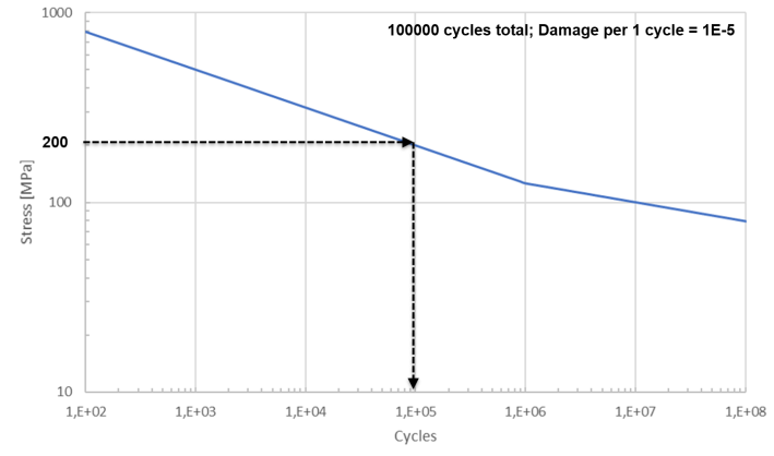
In the following example, a component is stressed with a stress range of 200 MPa. For this stress, the Wöhler curve defines a number of cycles to failure of 100,000 (1E5) cycles. Once cycle thus "consumes" 1/100,000 of the fatigue life. The Wöhler curve is plotted double-logarithmically.

As opposed to material tests, stresses on real components have almost arbitrary signal curves. Therefore, it is necessary to bin the time series of the measured signals in classes using a suitable method, which can then be converted to the damage domain and accumulated according to the above Miner method.

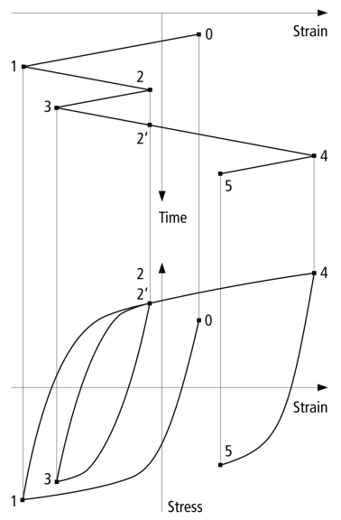
M. Matsuishi and Tatsuo Endo presented a method in 1968 – the rainflow cycle count – that represents the time signal on a time axis rotated by 90°. The method got its name from the similarity to a pagoda roof, over which rain runs off at the reversal points. First of all, half cycles, e.g. in the pulling direction, are counted and combined with matching half cycles in the opposite stress direction, e.g. pushing direction, to form closed cycles. This method is standardized in ASTM E 1049-85 (Standard Practices for Cycle Counting in Fatigue Analysis) and is in widespread use.

Determination and meaning of Wöhler curves

To determine the Wöhler curve, material samples with a defined sample geometry (frequently a round sample with a diameter of 10 mm) are clamped in a testing machine. The testing machine introduces cyclic forces into the sample, usually oscillating symmetrically around the zero value (mean stress-free) with a constant maximum force. However, variations in the cyclic compressive or tensile range are possible in order to determine material parameters with other mean stress values. The test is executed at a constant maximum amplitude up to failure (= fatigue fracture) or up to the technical incipient crack and the number of cycles reached for this load stage are entered in the diagram.

A material reacts in the case of an external stress, i.e. the introduced force F, on account of its geometry with cross section A, with a stress that is defined as the mechanical stress. With a known (initial) sample diameter and a known acting force, the resulting component stress can thus be determined as the quotient of F and A. It is usually specified in the unit Megapascal (MPa).

Accordingly, a mechanical stress value is plotted in the Wöhler curve over the achievable number of cycles. In order to determine the natural variance of the tests, several repetitions are carried out per load stage with equivalent material and the same sample geometry.

The execution of fatigue strength tests is standardized in DIN 50100 among others. The ASTM has also published a standard procedure for fatigue tests with constant amplitude in ASTM E466-15.

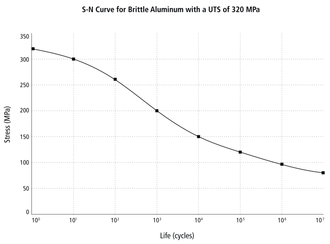
By way of example, a Wöhler curve for aluminum in a simple logarithmic representation is shown in the following.

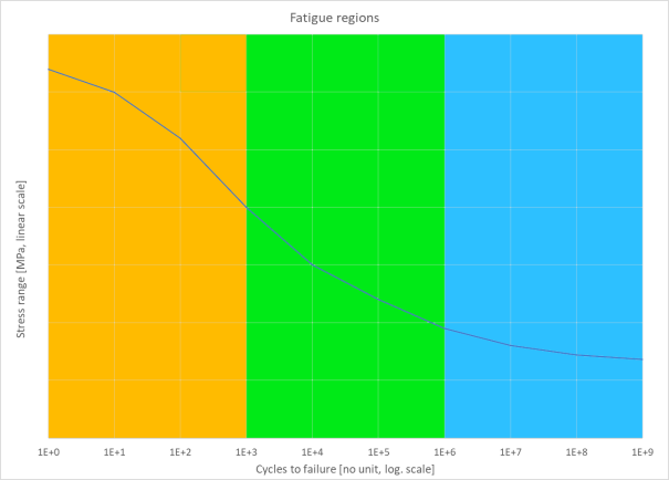
The Wöhler curve can be divided into three areas:

Low Cycle Fatigue, LCF: Area of high stress amplitudes
(N = 1 … approx. 10^4 cycles). Shown in yellow in the graphic below.

• High stress takes place in this area, in which strong plastic deformation of the material occurs. In this area, strain-controlled material tests illustrate the behavior much better, so-called strain Wöhler lines are used.
• In practice, only a few components are designed for the low cycle fatigue area.

High Cycle Fatigue, HCF: Area of a constant slope when the Wöhler curve is plotted logarithmically in the x and y-axes ([N = approx. 10^4 … 10^6). Shown in green in the graphic below.

• Classic area of operationally reliable component design.
• In widespread use in industry and research and in many applications.
• Many material parameters available in literature.

Very High Cycle Fatigue, VHCF: Area with no significant drop of the Wöhler curve from a certain amplitude [N > approx. 10^6]. Shown in blue in the graphic below.

• Theoretical stress limit below which no fatigue is observed (nevertheless, signs of fatigue appear e.g. due to corrosion and high temperatures).

A usable approximation of a Wöhler curve on the basis of the above three areas is illustrated in the following. For this, the Wöhler curve is converted to a double logarithmic representation, which is then subdivided into three linear sections. This representation is frequently used and can be created from just a few material parameters.

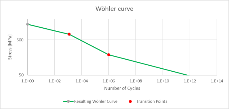
Common values for the slope k of the Wöhler curve are:

• Welded components: k = 3
• Electronic components: k = 4
• Components without stress concentrations: k = ~10

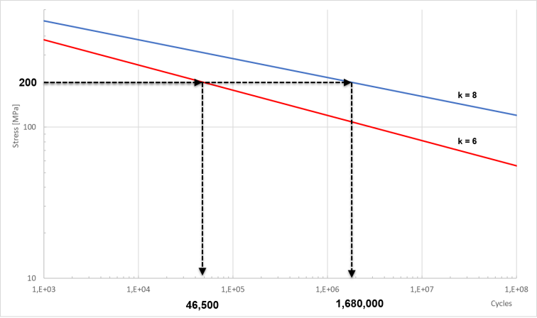
The flatter the slope of a Wöhler curve is (high k values), the less sensitive the material is in terms of its fatigue behavior. Smaller stress ranges thus cause less damage to the material, i.e. the tolerable number of cycles to failure up to a certain stress range is larger than with a material with a steeper slope of the Wöhler curve.

A steeper slope is suitable for components that are still susceptible to fatigue even with smaller stress ranges: welded constructions, components with stress concentrations or electronic components. In the following example, two Wöhler curves with the slopes k = 8 and k = 6 are plotted with the same stress intersection. The tolerable numbers of cycles to failure differ significantly (46,500 to 1.68*10^6).

Practical notes on interpreting the Wöhler curve

When working in the topical area of material fatigue, you should always bear in mind that the calculations are always of a statistical nature. Wöhler curves are frequently defined over a 50 % survival probability. This means that at the specified point of a p50 Wöhler curve, 50 % of the test specimens tested have already been destroyed. If a higher survival probability is required, curves with corresponding survival probabilities are to be derived from the material tests.

Not only the determination of the material parameters abstracts the scattered measurement results in a few simple curve parameters, but also material samples differ greatly from real components. In particular the shortened lifetime of components due to stress concentrations plays an important role.

Geometry:

• Test specimens have no sharp edges and are ground (no notches, blowholes, etc.)
• Sharp edges and punch-outs in the component cause local stress increases and cracking

Material quality:

• Test specimens have a high material quality
• The quality of real materials in production often fluctuates (blowholes, variation of manufacturing processes, oxidation, electrocorrosion, damage due to deformation, etc.)

Machining processes:

• Welded joints in real components
• Machining processes result in sharp edges, cut-outs and notches. Reworking of the surface or a design change can reduce these stress concentrations.

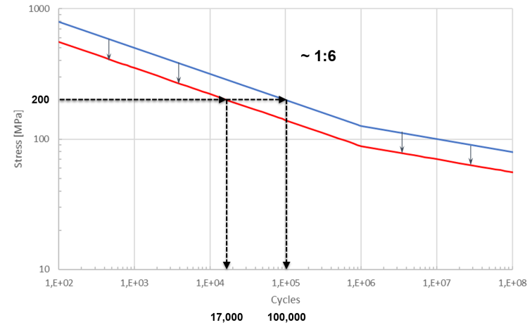
Stress concentrations lead to significantly earlier material failure. In the following, the influence of a stress concentration factor on the Wöhler curve is shown, which leads to a lowering of the curve and reduces the tolerable number of cycles to failure by a factor of 6.

If a precise statement on fatigue strength is required for a structural part/component, it is possible – depending on the component cost, size and availability of the component and test equipment – to determine a so-called "component Wöhler curve". In addition to the high costs for testing, the disadvantage here is that, although the significance for the current component is high, this can only be used to a limited extent if the component design changes.

Monitoring strategy: Fatigue or service life analysis

The load data is determined directly on the test specimen, e.g. by measurement with strain, force or pressure sensors. After the cycle counting with the rainflow algorithm, all the necessary information is available from the point of view of the loads. With regard to the fatigue assessment according to Miner, the material properties (Wöhler curve) are now to be consulted. The determination of the fatigue properties of the material used is often difficult, often there are few or no material characteristics available or they have to be estimated.

Practically, the following considerations help:

• Limitation to a relative comparison of identical components
• Use of literature data and corresponding conversion into an approximated Wöhler curve

Relative comparison of components

Generic Wöhler curves with defined slopes are suitable especially for relative comparisons of identical components, e.g. machine parts in series machine construction. The absolute damage sum is not meaningful here, but statements such as "Machine part B is 40 % more damaged than machine part A" can be derived and thus maintenance decisions can be supported.

Use of literature sources

For the determination of absolute damage values, Wöhler curves are usually determined from real material samples in testing machines. However, with Eurocode 3 and the FKM Directive, sources of material parameters of steel are also available from which Wöhler curves can be calculated.

In the following, stress ranges are always specified and not, as is usual in some sources, peak amplitudes. The stress range is twice as large as the peak amplitude.

The FKM Directive (Mechanical Engineering Research Curatorship, Association in the VDMA) specifies conservative material characteristics for different types and conditions of materials. An example from the FKM Directive (for more, see section Appendix).

Translation into the material parameters for the function F_CM_CalculateWoehlerCurve results in:

fSRI : LREAL := 4438;
fUTS : LREAL := 620;
bUseUTSCorrection : BOOL := TRUE;
fK1 : LREAL := 5;
fK2 : LREAL := 0;
nNC1 : ULINT := 18790;
nNC2 : ULINT := 1E+06;

fSRI and fUTS can therefore be directly applied. The slope is 5 as specified and refers to the area between the transition from the UTS correction to the very high cycle fatigue limit. The very high cycle fatigue limit is defined for NC, which is entered as nNC2. The slope in the very high cycle fatigue range is of course fK2 = 0. Only as an input into the function F_CM_CalculateWoehlerCurve, the transition point from the UTS correction to the area with slope 5 must additionally be calculated via the equation

.

Eurocode 3 (BS EN1993-1-9: 2005) defines different Wöhler curves for steel in different design details, in particular rolled/extruded products, welded and bolted connections and different geometries, such as T-beams. All Wöhler curves have these three section definitions in common:

• N ≤ 5*10⁶ where k = 3
• 5*10⁶ ≤ N ≤ 10⁸ where k = 5
• N ≥ 10⁸ where k=0 (not fatigue critical)

An example from Eurocode 3 (see section Appendix for more information).

A rolled or extruded product, manufactured as a plate, hollow cylinder or similar shape, is defined in the Eurocode as design detail 160.

Translation into the material parameters from the provided Fatigue Analysis results in:

fSRI : LREAL := 2580;
fUTS : LREAL := 20159;
bUseUTSCorrection : BOOL := TRUE;
fK1 : LREAL := 5;
fK2 : LREAL := 0;
nNC1 : ULINT := 5E+06;
nNC2 : ULINT := 1E+08;

The parameterization was converted here in such a way that the requirement for three defined zones with slope 3, 5, and 0 results when using the function F_CM_CalculateWoehlerCurve. The UTS correction is used here in such a way that a slope of 3 results in the first section. This is why fUTS is also larger than fSRI. The value for fSRI with k₂ = 5 is then

fUTS is then set to SRI from the Eurocode. This results in a slope of 3 in the first section. Setting fK1 = k2 and fK2 = 0 results in the other two sections.

Summary

The input values of a fatigue life analysis can be divided into three groups:

• Material properties describe the fatigue strength of the material, usually as a Wöhler curve, supplemented by surface texture and processing.
• Geometrical factors are used to adapt the material parameters to local geometrical properties that affect the fatigue life (e.g. notches or sharp edges).
• Loads are signals acting on the component that lead to stress. They are often measured with strain gauges or with force or torque transducers.

The analysis part contains the following components, depending on the degree of complexity:

• Corrections of material parameters and use of geometrical factors
• Cycle count for the conversion of time signals into classes (mean stress, stress range) for processing in damage accumulation
• Mean stress corrections to take into account the reduction of fatigue life due to mean stress effects
• Damage accumulation for the summation of the individual damage components from the cycle matrix, material parameters and correction factors

As a result, the damage sum is available for further comparisons, for example of identical components, or as a basis for warning/alarm messages. The monotonously increasing course of the damage sum is well suited for extrapolation to defined limits in order to identify critically stressed components and to be able to plan maintenance operations better.

This method is not only suitable for the classic fatigue analysis to calculate an absolute damage number, but also for relative comparisons of the damage intensity: Force or pressure signals, temperature cycles or other vibrating signal forms can be used to extend static methods (extreme values, crest factor, kurtosis, etc.) by meaningful information.

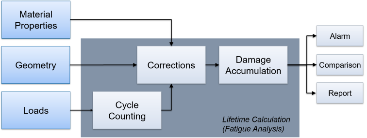
The three elements "Cycle Counting", "Corrections" and "Damage Accumulation", which are the central elements in the above graphic, are implemented in the TwinCAT 3 Condition Monitoring function with FB_CMA_RainflowCounting, FB_CMA_MeanStressCorrection and FB_CMA_MinersRule.

Appendix: Eurocode and FKM Directive

Eurocode 3 (EN 1993-1-9:2005 - Design of steel structures)

FKM Directive

The FKM directive specifies conservative material characteristics for different types and conditions of material. The following values for unalloyed structural steel, unalloyed fine grained structural steel, heat treatable steel and cast iron apply to a survival probability of 97.5 %.

Unalloyed structural steel

Tempered steel, tempered state