FB_TimeSync
This function block is used for system synchronization. The phase difference of the systems is determined based on the cycle index of received network variables, and a correction time is calculated.
Description
For synchronization of distributed systems the information is sent cyclically by one system and received by the others. Phase differences between the cycle times of the sender and the respective receiver lead to beat effects (see introduction) through information being missed or read twice. In the following section only the case with nominally identical cycle times on the sender and receiver side is considered. For different cycle times (even-numbered ratios are supported) the following description applies with different values.
Each send process is associated with a consecutive number, i.e. cycle index m of the network variables. The following cases may occur for the difference Δmi between the cycle index received during the current cycle (i) and the previous cycle (i-1) (Δmi=mi-mi-1):
Δm=0: The same data are read during the current and the previous cycle.
Δm=1: The sent data are received continuously.
Δm>=2: One or several pieces of information were not received.
Figure 1 schematically shows the case for Δm=0, i.e. duplicate reading of information, at the position indicated. Figure 2 shows case Δm=2, with sent information being skipped and not analysed.
Identification of beat effects
In the ideal case of times only differing through drift, the occurrence of Δm≠1 would indicate a step change. Due to the jitter of the cycle times around their nominal value, these cases predominantly occur around the beat, causing the step change to be broadened into a transition zone. The width of this zone depends on the magnitude of the clock jitter and on the absolute phase difference. Due to the width of the transition, it has to be identified through a condition that is different from Δm≠1. At discontinuities, deviations from Δm=1 cause the difference between sender and received cycles to increase. A difference that is constant over several (stTimeSyncParameters.iEndOfTransitionLimit) cycles is used for identifying the occurrence of a beat. This means that a step change can only be identified a certain number of cycles after its occurrence, which is significant for determining the corrections.
The phase difference between the computers is determined through the number of clock cycles of the receiver between two beats. This value can be used for correcting the beat effects.
Corrections
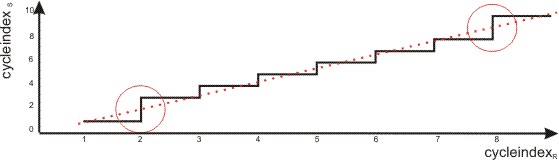
Figure 3 shows the cycle index of the sent information as a function of the received cycle index for case Δm=2 at the discontinuity. The beat effects cause the gradient of the curve to deviate from the ideal value of 1. In order to avoid step changes, a corrected cycle index can be calculated (dotted line) such that the beat effects are compensated during the time between the step changes. The result is a corrected cycle index on the receiver side that deviates slightly from the transmitted value, but is equidistant and shows no step changes.
Since discontinuities can only be detected after the event as described above, the correction calculated with the current drift can also only be applied with a delay. In order to avoid discontinuities of the corrected cycle index even in the event of strong differences in clock times, the drift used for the correction is gradually adjusted between the old valued and the new value once a discontinuity has been identified.
Another option for limiting the effects of strong changes in phase differences is non-uniform correction of beat effects, which means a stronger correction is applied after a discontinuity than just before the expected occurrence of the next discontinuity. If the time between two step changes becomes shorter, the correction is largely completed, and only minor additional corrections will be required. Further information can be found in the description of the configuration parameters.
Correction time
The correction time can be determined from the difference between the corrected and the received cycle index through multiplication with the cycle time. The correction time specifies the time shift required for the information currently being read, in order to enable equidistant interpretation without step changes. If the temporal variation of the value to be corrected is known, it can be extrapolated accordingly. For the cycle index the interrelationship is simple (+1 per cycle time), for extrapolation of axis information such as position and velocity, the velocity and acceleration have to be known (see documentation for function blocks FB_AxisSync and FB_AxisExtrapolateValues, and introduction).
Initialisation phase
For calculating the corrections, at least two beat effects must have occurred, in order to be able to calculate a drift. The so-called time mode is available for compensating fluctuations and step changes even before these two beat effects have occurred. In this mode (outputs bStartUp=TRUE and bSynced=FALSE) the corrected cycle index is incremented by 1 during each cycle, thus compensating step changes in the received cycle index. After a discontinuity has been identified (the time of occurrence of which is not yet foreseeable), the difference is compensated during the course of several cycles (stTimeSyncParameters.iTimeModeBlendingCycles). Once the required number of beats (stTimeSyncParameters.iNoOfPeriodsForMeanDrift) has been identified, the correction time is calculated according to the method described above (outputs bStartUp=FALSE and bSynced=TRUE), and the system changes from time mode to sync mode.
VAR_INPUT
VAR_INPUT
    iCycleIndex          : WORD;
    fTaskCycleTime       : LREAL;
    bEnable              : BOOL;
    stTimeSyncParameters : ST_TimeSyncParameters;
END_VAR
iCycleIndex : Cycle index of the currently received data
fTaskCycleTime : Nominal receiver cycle time in [s]. If the cycle time of the sender differs from this value, it has to be configured via parameter stTimeSyncParameters.fDataCycleTime. Otherwise it is assumed that both cycle times are identical. The cycle times must be even-numbered multiples of each other, i.e. tSender=2ms, tReceiver=4ms or tReceiver=1ms, for example.
bEnable : FALSE deactivates the function block, a rising edge reinitialises and starts it
stTimeSyncParameters :Structure contains the Configuration paramters
VAR_OUTPUT
VAR_OUTPUT
    bError              : BOOL;
    iErrorId            : DINT;
    bWarning            : BOOL;
    iWarningId          : DINT;
    fCorrectionTime     : LREAL;
    bSynced             : BOOL;
    bStartUp            : BOOL;
    stTimeSyncDiagnostic: ST_TimeSyncDiagnostic;
END_VAR
bError :TRUE in the event of a fault
iErrorId: Returns error code (E_Sync_ErrorCodes) in the event of a fault
bWarning : TRUE in the event of a warning, i.e. operation continues under sub-optimum conditions.
iWarningId : Returns the corresponding warning code (E_Sync_WarningCode)
fCorrectionTime : Correction time, i.e. the time used for extrapolating the received information [s]
bSynced : TRUE if sender and receiver are synchronised. The system was able to determine a correction time in sync mode, i.e. the initialisation phase is completed, and the correction time is within the permitted range (i.e. after identification of stTimeSyncParameters.iNoOfPeriodsForMeanDrift beats, and the absolute value of the correction time subsequently falling stTimeSyncParameters.fThresholdForSync*TaskCycleTime).
bStartUp : TRUE if the function block is in the initialization phase. During this phase the correction time is calculated such that it can be used for extrapolating the data, although _only_ fluctuations ( Δm≠1) are compensated. After identification of a beat during the initialization phase, a correction time of 0 is applied linearly withinstTimeSyncParameters.iExtendedStartUpBlendingCycles cycles.
stTimeSyncDiagnostic: Structure with advanced diagnostics outputs