Signal quality when outputting signals with digital analog outputs – distortion factor
The modular Beckhoff I/O system IP20/IP67 features analog outputs in various designs, e.g. the EL41xx, EL47xx, EJ4xxx or EP4xxx series ("xx" or "xxx" stands for the respective specific product number).
What all devices have in common is that they
- operate with electronic DACs (digital-to-analog converters): a digital value sent by the controller (TwinCAT) via the fieldbus, e.g. 4567dec = 11D7hex, is converted by the DAC per channel to an analog output (voltage or current, depending on the device) and possibly also amplified,
- operate cyclically: the controller sends its output values, time-discrete, in a fixed real-time rhythm ("control cycle"), e.g. every millisecond. The analog output device receives this value via the fieldbus and outputs it according to the set operation mode; three modes are available, depending on the device
- immediate output after reception: SyncManager-synchronous,
- triggered by the local clock: DistributedClocks-controlled,
- free-running: the device firmware continuously repeats its MAIN loop and outputs the received value according to its own requirements.
Overall, this means that a smooth signal curve cannot be produced, and instead a stepped (in terms of time and amplitude) signal curve is seen at the output (particularly if there is no internal or external signal smoothing):
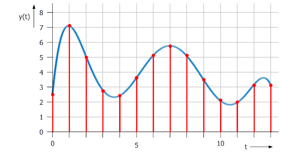 Fig.50: Analog signal (schematic, discretized)
The actually specified analog signal (blue) can only be electrically mapped by dedicated interpolation points (red dots). As a result of this, the real output signal is stepped both in the time dimension and in the amplitude dimension – it is discretized.
See the following example with the EL4732 (analog output ±10 V, max. 100 kSps, oversampling-capable):
- for the output of a sinusoidal signal, the following TwinCAT 3 PLC code is used, in which sine values are calculated for the configured oversampling field for each calling cycle:
Declaration:
   FUNCTION_BLOCK FB_sine_generator
   VAR CONSTANT
       // TwinCAT / Terminal configuration:
       CnMaxIdx           : UDINT  :=10;    // Fixed amount for Oversampling
       tCycleTime         : LTIME  :=LTIME#1MS; // Configured task cycle time
       nOversampling      : UDINT  :=10;    // Used oversampling of the terminal
   END_VAR
   VAR_INPUT
       // Output configuration:
       rFreq_Hz           : LREAL   :=1;    // Destination frequency
       rAmplitude         : LREAL   :=1;    // Destination amplitude
   END_VAR
   VAR_OUTPUT
       bError             : BOOL;
       arOut              : ARRAY[1..CnMaxIdx] OF LREAL;
       aiOut_EL4732 AT%Q* : ARRAY[1..CnMaxIdx] OF INT; // 10 V max
   END_VAR
   VAR
      nIdx                : UDINT;
      rPosition            : LREAL := 0;   // Init, if for startup important
      rPeriod_Sec,
      rStep,
      rPositionPi,
rValue : LREAL; END_VARExecution:
// This code generates values of a sinus for an EL4732 analog output terminal
   IF nOversampling > CnMaxIdx OR (nOversampling = 0) OR
    (tCycleTime = LTIME#0S) THEN
       bError := TRUE;
   ELSE
       bError := FALSE;
       rPeriod_Sec := 1 / rFreq_Hz;

       // Calculate a step width (percentual of 1):
       // Divide the cycletime by the destination periode and ovs factor:
       rStep := (1E-9 * LTIME_TO_LREAL(tCycleTime))
                  / (rPeriod_Sec * UDINT_TO_LREAL(nOversampling));
       // (Note:
       // factor of 1E-9 for value in seconds due to LTIME data type's unit is ns)

       // fill the array bound to oversampling output for one task cycle
       FOR nIdx := 1 TO nOversampling DO

           // Calculate next X-Position of the sine:
           rPosition := FRAC(rStep + rPosition);
           // (usage of FRAC for saturation of rPosition to < 1)

           // Calculate percent from 1 to an angle of radians:
           rPositionPi := (rPosition * 2 * PI);

           // Calculate next Y-Value:
           rValue := rAmplitude * SIN(rPositionPi);
           arOut[nIdx] := rValue; // allocate to array

           // Convert output to PDO of EL4732:
           aiOut_EL4732[nIdx] := LREAL_TO_INT((rValue / 10) * 16#7FFF);
       END_FOR
END_IF | Using the sample programs This document contains sample applications of our products for certain areas of application. The application notes provided here are based on typical features of our products and only serve as examples. The notes contained in this document explicitly do not refer to specific applications. The customer is therefore responsible for assessing and deciding whether the product is suitable for a particular application. We accept no responsibility for the completeness and correctness of the source code contained in this document. We reserve the right to modify the content of this document at any time and accept no responsibility for errors and missing information. |
Explanation of the example
- with cycle time = 1 ms, oversampling = 10, amplitude = 1 V and f = 758 Hz, the ScopeView displays the following image of the PLC variable arOut:
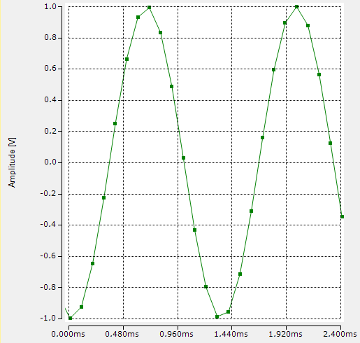
The individual calculated interpolation points can clearly be seen (setting of the channel property: property group "Marks", property "Mark State" = On, "Mark Size" = 4). - The preset channel property "Graph Type" under the property group "Line" in the scope is preset to the representation "Line". For that reason, the above ScopeView output does not correspond to the actual electrical output signal of the terminal. A change in the "Stair" representation comes closer to that:
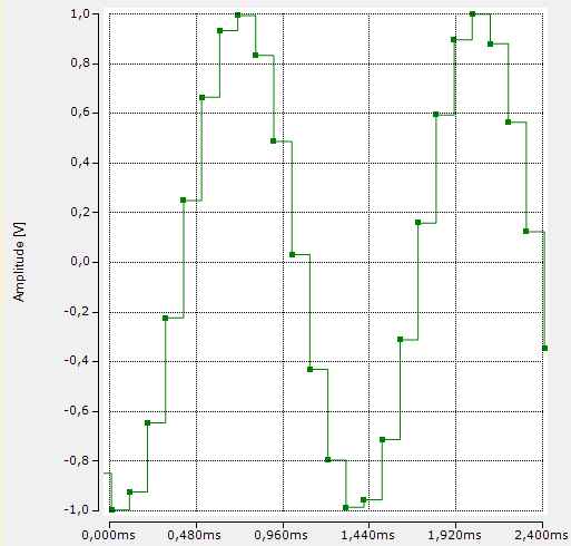
this "Graph Type" can selected as shown below: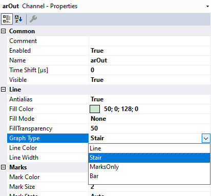
- For that purpose the electrical signal that in reality leaves the analog device, which operates digitally and is thus discretizing in the time and amplitude dimensions, is recorded with an oscilloscope EL4732/Ch1 across a load of 1 kΩ:
 .
. - The resolution in the time range (x-axis) depends on the configured task cycle time (CycleTime) and the set oversampling factor (Oversampling):
Resolution [s] = CycleTime / Oversampling
With the above values, 1 ms/10 = 0.1 ms. The number of consecutive analog values per second results from the reciprocal value of the resolution: hence, in this example (1 ms cycle time, 10-fold oversampling), 10,000 consecutive analog values can be output with a resolution of 100 µs (colloquially "output at 10 kHz").
So much for the theory. Now, in some tasks the question may arise as to the analog signal fidelity in relation to the theoretical signal. There are various evaluation criteria for this, for instance the distortion factor.
For sinusoidal signals, the distortion factor states the harmonic content of the real signal in relation to the total signal, in other words the magnitude of the contents in the signal that do not correspond to the ideal sine wave, i.e. that distort it. The distortion factor lies between 0 and 1; in general, a low distortion factor close to 0 shows a real signal that is very close to an ideal sine wave and contains few (undesirable) harmonics.
 Fig.51: Distortion factor: ideal sine, output, measurement and evaluation
Measurement and evaluation as follows:
- output of the sinusoidal signal across a known load,
- measurement with the oscilloscope and FFT evaluation,
- determination of the RMS value of the integer harmonics, and from that
- the calculation of the distortion factor.
In the following example, this distortion factor calculation is to be performed on the sinusoidal output of an EL4732 (±10 V, 10 kSps per channel), where f = 1 kHz and RLoad = 1 kΩ.
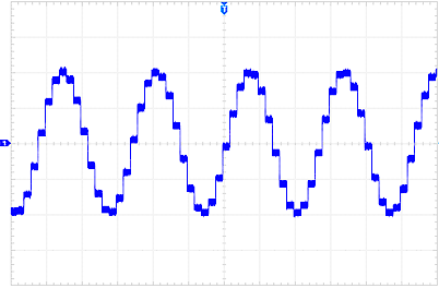
A simple oscilloscope with FFT function is used: the 1 kHz sinusoidal signal can be seen in the time range (blue) with 10-fold oversampling:
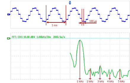 Fig.52: Sinusoidal output signal of the EL4732 and FFT evaluation
The FFT evaluation is green. The RMS values [dBV] read from this (note: observe the base line "M") and converted to Vrms = 10-(dBV/20) are as follows:
Frequency [kHz] | RMS value [dBV] | RMS value [Vrms] |
|---|---|---|
1 | -4 | 0.630 |
2 | -51 | 0.0028 |
3 | -46 | 0.005 |
4 | -60 | 0.001 |
5 | -53 | 0.002 |
According to the equation:
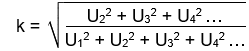
a distortion factor of 0.92% results.