Description of the visualization
The visualization for the editing of two EL3351s has the following appearance as standard:
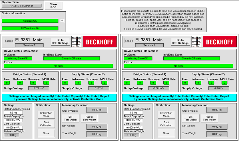 Fig.168: Main page of the visualization
Clicking on the "Go to CoE Settings" button on the "Main" page during operation takes you to the page on which the CoE entries can be set. A small example of RGB color editing is opened by clicking on the "Show RGB" button.
System Time
The current Windows system time is displayed in this field.
Status information
The upper text field displays the status of the EtherCAT device. For further information see: EtherCAT Master Diagnostics
The second text field indicates whether an error has occurred in the terminals during operation. If this is the case, the number of the terminal in which the error has occurred is displayed.
Device status information
The status of the terminal is displayed here. The field with the label "WcState" displays the status of the working counter.
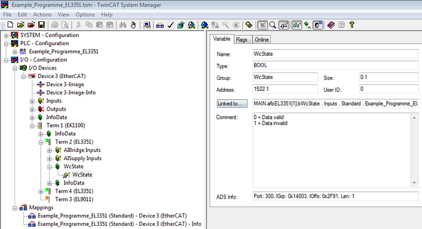 Fig.169: Working Counter EL3351
As soon as WcState adopts the value "1", the terminal is no longer participating in the process data traffic. If valid real-time communication is taking place, WcState has the value "0".
The "InfoData State" field displays the status of the terminal.
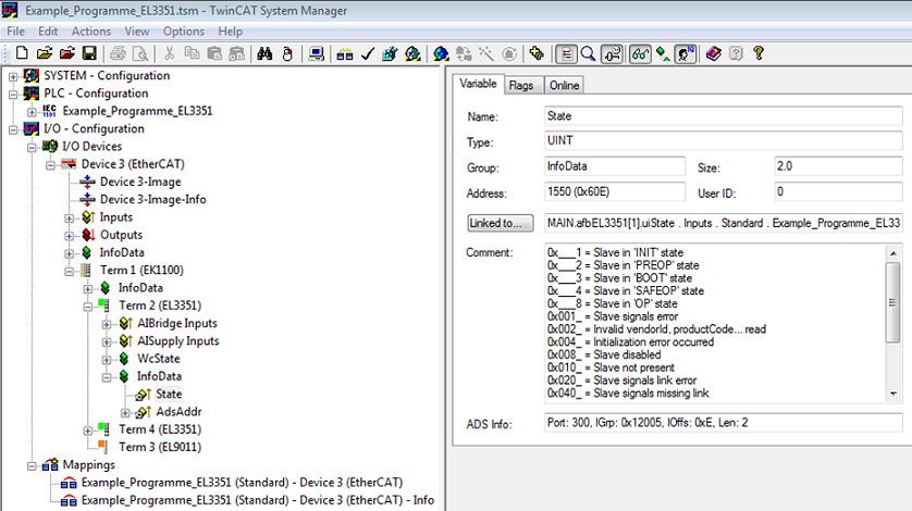 Fig.170: State EL3351
If this status is not equal to 8, then the terminal is not in the OP (operational) status. Information about which different statuses the value can adopt is provided by the Infobox in the System Manager (see fig. State EL3351).
Bridge Status/ Supply Status
This area informs you about the status of the channels for the acquisition of the bridge voltage and the reference voltage. The individual values take the form of Boolean variables. There is an error if the value "1" is adopted.
Visualization - Main
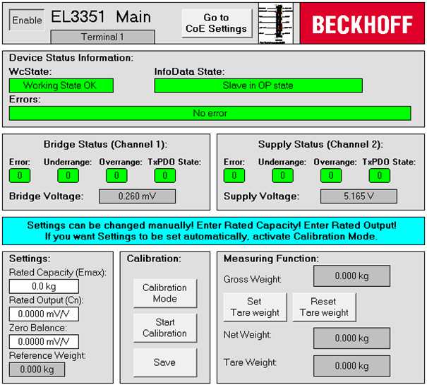 Fig.171: Visualization example program for EL3351, main page
Bridge Voltage/ Supply Voltage
The size of the measuring signal UDiff in mV and the reference signal URef in V are displayed in this area.
Settings
The nominal characteristic value and the nominal load of the connected load cell must be set at the beginning. Clicking on the respective field enables a value to be entered. The input of a zero error (zero balance) is optional.
Calibration
Clicking on the "Calibration Mode" button activates the calibration mode. This mode permits the automatic determination of the size of the zero error and the nominal characteristic value of a connected load cell. If the mode is activated, instructions appear in the text field of the visualization to guide you through the entire calibration process. The calibration is started by clicking on the "Start Calibration" button.
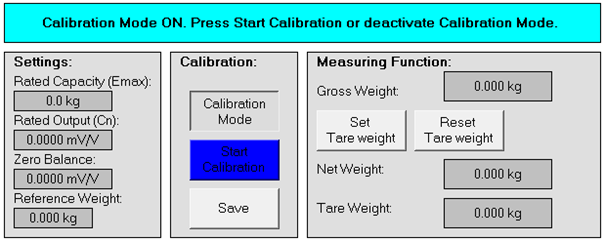 Fig.172: Calibration mode: Start
If it has not already been done, the nominal load of the connected load cell must be entered first.
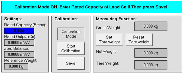 Fig.173: Calibration mode: Input of nominal load
If this has been done, the next step is initiated by pressing the "Save" button.
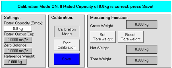 Fig.174: Calibration mode: Confirmation of nominal load
The zero error of the load cell is now determined. It must be ensured when doing this that the load cell is not loaded. If this is the case you can move to the next step with "Save".
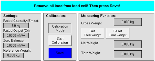 Fig.175: Calibration mode: Determining the zero error
In order to determine the nominal characteristic value, the load cell must be loaded with a known reference weight. The higher and more precise the reference weight is, the more precise the nominal characteristic value will be. The reference weight must be entered into the associated field.
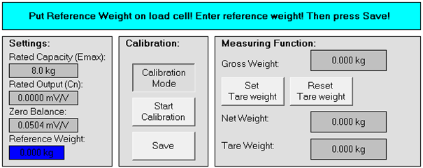 Fig.176: Calibration mode: Entering the reference weight
The calibration process is concluded by pressing the "Save" button.
The size of the calculated nominal characteristic value and zero error can be taken from the respective fields under Settings.
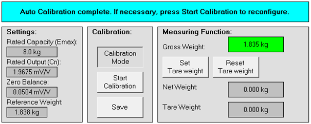 Fig.177: Calibration mode: Conclusion
A new calibration can be started by pressing the "Start Calibration" button. If the calibration mode is ended by clicking on the "Calibration Mode" button, the calculated settings are retained.
Measuring Function
On basis of the functions provided in the example program, the weight loading the load cell is calculated from the values for the nominal load, the nominal characteristic value, the measuring signal and the reference signal and - if it exists - from the zero error. The tare weight can be set via the "Set Tare weight" button if a weight is loading the load cell. The set tare weight is deleted by pressing the "Reset Tare weight" button. If a tare weight is set, the net weight is calculated using the equation net weight = gross weight - tare weight.
 | Supply voltage and characteristic value of the load cell The supply voltage of the load cell should be selected to suit its characteristic value. The maximum measuring range of the measuring signal is +/- 20 mV. If the load cell has a characteristic value of 2 mV/V, for example, then a supply voltage of 10 V should be selected so that the maximum differential voltage is 20 mV/10 V. If the load cell used has a nominal characteristic value of 4 mV/V, the 5 V supply voltage can be picked up directly at the terminal, for optimum utilization of the measuring range (as described in Fig. Connection of a load cell with 5 V supply via the EL3351). |
Visualization - CoE
The CoE entries can be read and modified on page 2 of the visualization of the example program.
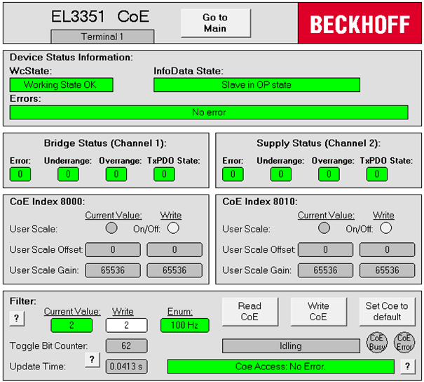
Fig. 31: CoE page of the visualization
Clicking on the "Go to Main" button on the "CoE" page during operation takes you to the page on which the weight calculation takes place.
CoE Index 0x8000 / 0x8010
At this point "User Scaling" can be activated and the offset and gain of "User Scaling" can both be adjusted. Values can only be entered if "User Scaling" is activated. This is done by clicking on the On/Off button. The changes are confirmed by pressing the "Write CoE" button.
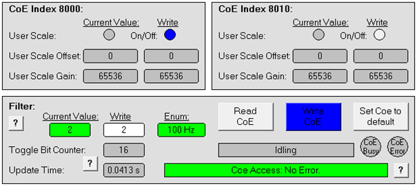 Fig.178: Activation of "User Scaling"
After activating "User Scaling" both the offset and the gain can be adjusted. All changes must be confirmed by pressing the "Write CoE" button.
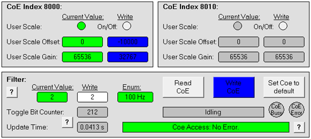 Fig.179: Input of offset and gain
Button "Read CoE"
Pressing this button causes the CoE entries in the indices 0x8000:0 and 0x8010:0 to be read out successively and their values displayed on the visualization.
Button "Write CoE"
If you wish to modify CoE entries, you must enter the changes via the display elements. The changes are confirmed by clicking on the "Write CoE" button.
Button "Set CoE to Default"
Actuating this button causes all CoE entries to be reset to the factory preset values and directly written.
Filter
The filter setting determines the filter frequency and thus the conversion time for both channels of the terminal. The higher the filter frequency, the faster the conversion time. Furthermore, the toggle bit is evaluated over a period of 10 seconds. A new set of process data is present on both a rising and falling edge. An example of this is given in the section TwinCAT Scope View 2 demonstration. The update time is calculated directly from the number of rising and falling edges of the toggle bit.
Dealing with real characteristic values
The nominal characteristic values of load cells are subject to tolerances which can be taken from the associated certificates. Hence it could be the case, for example, that the nominal characteristic value of a load cell is specified as 2 mV/V, but deviates slightly from that according to the certificate. In addition to that there is a zero error in most cases.
The following is intended to describe how the example program can be adjusted with these values. The data of the load cell in this calculation example should be as follows:
- Reference voltage: 5 V
- Nominal characteristic value: 2.12 mV / V
- Zero error: 0.046 mV / V
First of all the real nominal characteristic value can be entered in the "Rated Output (Cn)" field and the zero error in the "Zero Balance" field. Another possibility to compensate the zero error is to employ the user scaling. The associated value must be entered in the "User Scale Offset" field. The following calculations must be performed in order to obtain the value that balances the zero error from this example:
The following maximum differential voltage results from fully loading the load cell:
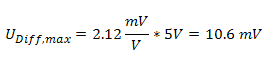
The raw value of the measuring signal at 20 mV/V is 2147483647. Hence, the maximum raw value that can be achieved with a measuring signal of 10.6 mV is:
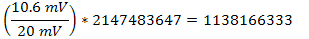
From this, the raw value of the zero error becomes:
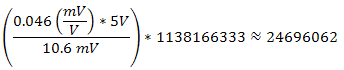
In order to compensate this error, the zero point must be "shifted downwards" by precisely this value; hence, "- 24696063" must be entered in the User Scale Offset field.
Visualization - RGB
A small example of RGB color editing is opened by clicking on the "Show RGB" button. The color in which the text field with the instructions appears is dynamically composed of the basic colors red, green and blue. The values of these three colors are shown in this window, as is the combined value of all three colors. The red, green and blue components can be adapted using the regulators and the combined color appears in the lowest field.
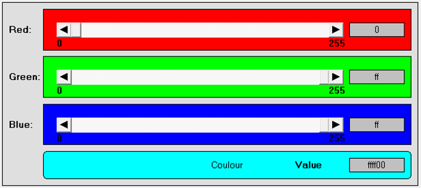 Fig.180: RGB window