Calculating the synchronisation phase
An attempt is made when calculating the synchronisation phase to find an optimum solution while observing the boundary conditions specified by the user. If it is not possible to observe the specified boundary conditions, the coupling is declined and an appropriate error message is issued.
Optimizations
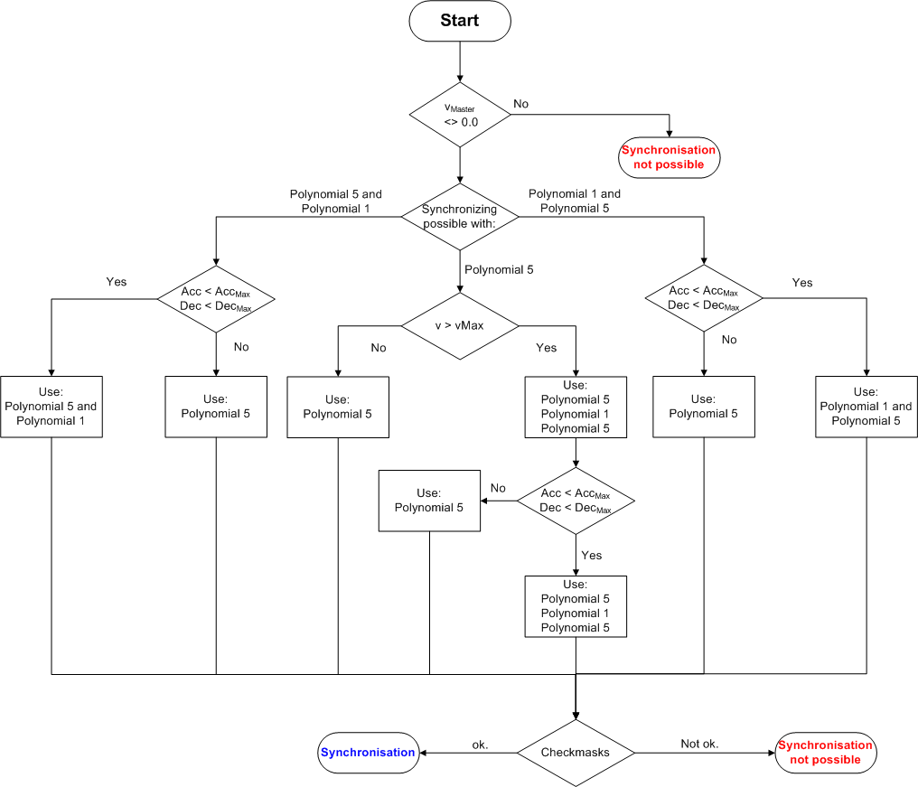
As can be seen in the flow chart below, the individual bit masks partly influence the internal optimization steps of the profile calculation, since an optimum is searched for depending on predefined rules (see Parameterizable boundary conditions). Essentially, a 5th order polynomial or a combination of a 5th order polynomial with a 1st order polynomial is used. A 5th order polynomial is generally not free from overshoot, but the accelerations are more moderate than when combining a 5th order polynomial with a 1st order polynomial. The combination of the 1st and 5th order polynomials is calculated in such a way that it is always free from overshoot. However, higher accelerations and decelerations occur with it. If, for example, the actual velocity matches the synchronous velocity, but a certain position difference must be compensated. Then the optimum velocity is calculated internally as a function of the maximum acceleration. Result is a 5th power polynomial a 1st order polynomial with the calculated velocity and a 5th power polynomial. At least one of the two 5th power polynomials exploits the maximum acceleration. To avoid extreme jerk values, the jerk check should be switched on.
 | The optimizations shown can only be carried out if both the master and slave axes are free of acceleration at the time of coupling. For accelerated axes, a 5th order polynomial is used for synchronization, which is checked for compliance with the specified boundary conditions, but cannot be optimized. |
Notice | |
If the master axis is an encoder axis (an "external encoder system"), something which as a rule is never mathematically free from acceleration, particular care must be taken to filter the actual acceleration. Alternatively the determination of the actual acceleration can be deselected in the encoder, i.e. set to zero. The NC also has an internal algorithm for this combination (master encoder axis with the Universal Flying Saw as a slave). This algorithm sets master accelerations whose magnitudes are less than (2.0 • scaling factor / cycle time2) to zero at the coupling time. |
Optimisation step 1:
Aim: "Velocity profile free from undershoot or overshoot"
An attempt is first made to calculate a profile that synchronises the velocity without overshoot or undershoot (a combination of a first order polynomial and a 5th order polynomial or vice versa: in abbreviated form, polynomial1+polynomial5 or polynomial5+polynomial1). If the acceleration check is active at this stage, and if one or more of these limit values (acc, dec) is exceeded, then another profile, which in general is not free from overshoot (polynomial5) is calculated. If one of the active limit values (acc, dec) is still exceeded with his profile, then the synchronisation command is finally declined with an error code.
Optimisation step 2:
Aim: "Limitation to maximum permitted velocity"
If the first optimization step is not possible, the second optimization step checks whether the maximum permitted velocity for the slave axis is exceeded by a general standard profile (polynomial5). If this is the case, an attempt is made to generate a profile in which the maximum profile velocity is precisely the maximum velocity permitted to the slave axis (machine data) (polynomial5+polynomial1+polynomial5). It should be noted that this optimization attempt usually results in larger values of acceleration or deceleration.
If the acceleration check is active at this stage, and if one or more of these limit values is exceeded, then this second optimization step is rejected, and finally a profile, which is not in general free from overshoot (polynomial5), is calculated. If one of the active limit values (acc, dec) is still exceeded with his profile, then the synchronization command is finally declined with an error code.
Optimisation flow diagram:
The optimizations carried out internally are illustrated in the following flow diagram. Essentially, the slave set value profile is calculated as a 5th order polynomial. This 5th order polynomial can be combined with a first order polynomial in order to maintain the parameterized boundary conditions. The way in which the individual boundary conditions influence the selection of the polynomials, and therefore the form of the set value profile, can be seen from the flow diagram illustrated below. The label "polynomial n and polynomial m" expresses the fact that polynomial n is first used in the synchronization phase, followed by polynomial m.