Task Setting
Applications with several real-time tasks
A Condition Monitoring analysis chain is made up of the data collection, usually several algorithms and the provision of the results. The further processing of the results as well as the reactions of the program to these depend on the application.
Since the scope of the input data, e.g. the length of input vectors, strongly depends on the respective application, signal processing software requires arrays with different lengths and different element types. Therefore the TwinCAT 3 Condition Monitoring Library uses a flexible data structure throughout for numerical arrays. This allows numerical data to be saved, transferred and evaluated block by block. It can represent both multi-dimensional and one-dimensional data.
The Condition Monitoring algorithms are very CPU-intensive depending on the configuration. The algorithms are therefore preferentially outsourced to a separate task. In this case the analysis chain extends over several tasks. The associated difficulties of synchronous data exchange and thread security are internally encapsulated by the library function blocks in order to enable flexibly manipulable analysis chains.
Further information on data exchange can be found in section “Parallel processing”.
Tip: Of course, the program can also be implemented as an application of a single task. This is recommended if the required algorithms can be processed fast enough, depending on the CPU and the task cycle time.
Task cycle times
The analysis steps and the corresponding buffer sizes represent a condition for the task cycle time. The calculation must be performed often enough to be able to process all input data.
Sample: The data collection is stored in buffers, the size of which was declared as 1600 elements. With an oversampling rate of 10x, a buffer takes 160 cycles to fill. If the signal collection is triggered by a 1 ms task, the task calculation must be triggered with a cycle time of less than 160 ms.
It is recommended to set the calculation cycle time to a lower value, in order to realize a faster response (at least a factor of 0.5). On the other hand, the smallest possible calculation cycle time depends on the complexity of the algorithms to be calculated and the performance of the CPU used.
 | Guide value for the upper limit of the calculation cycle time Calculation cycle time < 0.5 * signal collection cycle time * buffer size / oversampling rate |
Most algorithms (spectrum, cepstrum,...) contain computationally intensive mathematical operations. They should be called in a task context with sufficient cycle time. The required execution point also depends on the hardware platform. The above equation represents an upper guide value for the calculation cycle time. For example, a profiler is provided for each function block for estimating a lower guide value, which can be activated during online monitoring. You can find this profiler in the instance of the function block under fbImplementation → fbExecutionTimeMonitoring. By manually setting bMeasureMeasureMaxExecTime you activate the profiler. As usual, you do not want to access internal variables of a function block programmatically.
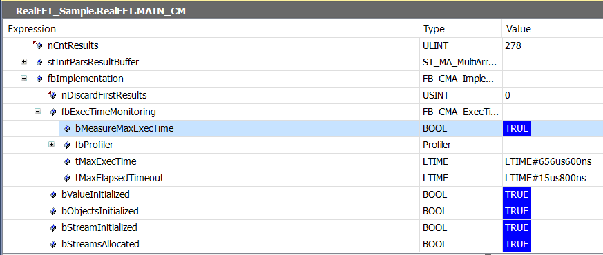
The displayed values are maximum execution times. The task settings should provide a small reserve for possible combinations of parameters and input values that could lead to longer execution points.
Exceptions to the above considerations are some statistical function blocks (quantiles, histograms,...). As a rule, these function blocks initially only add data for several task cycles to the internal memory. Only the subsequent calculation (collecting data after N cycles) takes time. The corresponding task cycle time can be adapted to the simple call without calculation. While this leads to exceeding of the cycle time in the event of calls with calculation, it ensures fast response times. This is a special case for PLC programming. Normally, a task cycle time should never be exceeded.
| Note the cycle time The cycle time of tasks, which only call Condition Monitoring algorithms, can be adjusted in such a way that the cycle time is rarely exceeded. Program blocks, which are called by this task, should not contain other program code! And the priority of these slower tasks should, of course, be lower than that of other tasks. |
Floating point exceptions
These exceptions can be disabled separately for each task. They are enabled by default.
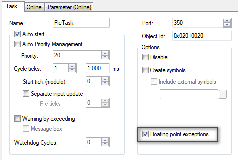
Some algorithm calls can lead to a NaN (not a number) result. If NaNs are to be processed in the application, the FP exceptions have to be disabled for this task. Then, you must verify that the whole program code and all functions can handle NaNs.
Further information regarding the handling of NaN values can be found in the separate section “NaN values”.
| |
Execution stop Floating point exceptions are active by default. Comparisons with NaN (Not a Number) can cause such an exception that leads to an execution stop and may possibly cause machine damage. It is urgently recommended to check the result for NaN before it is processed. (see section “NaN values”) |
