Example 6

The procedure for creating a motion diagram is illustrated in this simple example.

The task:

The following slave motion is to be implemented for a rotation of the master axes from 0 to 360 degrees.

• In the tree structure, create a master and its corresponding slave via MOTION > Tables (see Introduction).

• After selecting Slave 1 in the tree structure, both the graphic window and the table window appear.

• In the graphic window, click the approximate positions of the points in the window using the Insert Point command.

The corresponding values will then be inserted into the table window.

• To turn the motion plan into a motion diagram, you now need to add some information.

• For the first, third and fifth sections we use the Synchronous Function command to specify by clicking with the mouse in the corresponding sections that a linear motion should take place there. In the second and fourth sections, the function type is defined in the table as an 8th order polynomial.

• In the second section in the table, select the function type acceleration trapezoid from rest to turn (AccTrapezoid_RT: Rest in Turn) and in the third section as acceleration trapezoid from turn to rest (AccTrapezoid_TR).

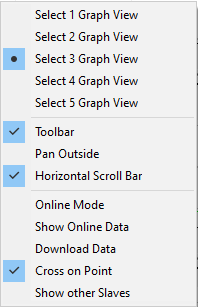
By right-clicking and selecting Select Graph 3 View, the velocity in the second graph window and the acceleration in the third graph window are displayed in addition to the slave position in the first graph window.

The size of the windows can be changed interactively by positioning the mouse on the edge and moving it with a left click.

• To ensure that the exact positions are realized, enter them now in the table view.