Digital filters
Digital filters are used to manipulate digitalized (time-discrete and value-quantized) signals. The manipulation is evident in the frequency domain, where certain components of a signal are emphasized or suppressed.
Properties
Digital filters can differ, among other things, in the frequency domain that may pass through the filter.
Filter type | Description | Area of application (examples) |
|---|---|---|
Low-pass | Frequencies below a cut-off frequency can pass through the filter. | Anti-aliasing filter or filter for smoothing a signal. |
High-pass | Frequencies above a cut-off frequency can pass through the filter. | Elimination of an interfering DC component in the signal. |
Band-pass | Frequencies within a certain frequency interval can pass through the filter. | Useful for amplitude-modulated signals (radio technology, optical measuring signals, ultrasound signals, ...), i.e. the wanted signal is spectrally distributed around a carrier frequency, so that low and high frequencies outside the wanted signal worsen the SNR (signal-to-noise ratio) and are suppressed. |
Band-stop | Frequencies out of a certain frequency interval can pass through the filter. | Suppression of an inductively coupled frequency, e.g. the mains frequency. |
The specific implementation of the filter determines the transition behavior from the passband to the stopband.
See also: Filter types and parameterization
Digital signals
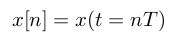
An analog signal x(t) is converted by an analog-to-digital converter, e.g. in an EL3xxx or ELM3xxx, to a time-discrete and value-quantized signal x[n]. The time discretization takes place with the sampling period T (inverse of the sampling rate fs).
|
Difference equation
The general difference equation for an input signal x[n] (input to a discrete system, in this case a filter) and a corresponding output signal y[n] is:
|
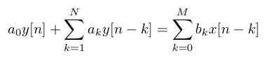
ak und bk are usually real-valued coefficients (filter coefficients). The current output value y[n] of a system is thus calculated as a linear combination of past filter inputs x[n-k] with k > 0, past filter outputs y[n-k] with k > 0 and the current filter input x[n] (k = 0).
The inclusion of past filter outputs in the calculation of a current output value represents a feedback and therefore requires verification to ensure system stability. Filters with feedback are called "IIR filters" (Infinite Impulse Response filters). Filters without feedback are called "FIR filters" (Finite Impulse Response filters). The advantage of IIR filters is that "good" manipulations of the signal x[n] can be achieved with low filter orders. By definition, FIR filters can never be unstable.
Transfer function
By z-transforming the difference equation and using the linearity and the time shift property, the following general representation of the filter transfer function is obtained:
|
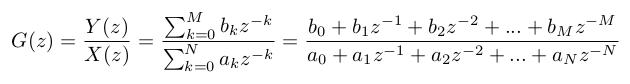
The denominator coefficients ak belong to the coefficients in the feedback. In order for the filter to be stable in conjunction with the transfer function G(z), care must be taken when calculating these coefficients that the poles of G(z) lie within the unit circle in the complex level.
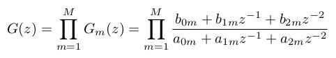
IIR filters with a high filter order can become instable due to quantification effects during the calculation of the coefficients. In order to overcome these challenges, IIR filters are often implemented in cascaded biquad filters, normally called second-order sections (SOS). The overall transfer function is expressed by a multiplication of several 2nd order filters. The transfer function G(z) is then described with:
|
The frequency response of a system can be determined from the transfer function G(z) by transitioning to the frequency range (frequency f) with 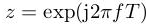 . The amplitude response then corresponds to the magnitude of the frequency response, and the phase response corresponds to the argument of the frequency response.
Implementation in the PLC library
The PLC library Tc3_Filter provides various function blocks for implementing digital filters.
The function block FB_FTR_IIRCoeff can be used to implement a free filter. The filter coefficients ak and bk can be calculated individually and transferred to the function block using a configuration structure. You are responsible for the stability of your filter.
With the function block FB_FTR_IIRSos you can implement a free filter structured in SOS. The filter coefficients ak and bk can be calculated individually and transferred to the function block using a configuration structure. You are responsible for the stability of your filter.
The function block FB_FTR_IIRSpec can be used to implement ready-made filters of type Butterworth, Chebyshev or Bessel through simple parameterization. The filter coefficients are thereby calculated internally as biquads.
The function block FB_FTR_MovAvg and FB_FTR_Median can be used to implement an average filter or median filter, which is used in many applications for smoothing signals.
Use the function block FB_FTR_Gaussian to create a smoothing filter with minimal group delay so that the shape of your signal is only minimally affected as it passes through the filter and only the interfering signal components are removed.
You can use the function block FB_FTR_Notch to implement a band-stop filter that is used to suppress a narrow frequency band.
You can use the function block FB_FTR_ActualValue to perform a plausibility check of a measured input value.
In addition, further filters that are commonly used in system theory and control technology are made available to you: PTt, PT1, PT2, PT3, PTn, PT2oscillation and LeadLag elements.
A PT1 element and a Butterworth 1st order low-pass filter can be converted equivalently to each other, but the featured parameters of the filters are different.
Bilinear transformation
The parameterization of the predefined filters takes place in the Laplace space. The implementation of the time-continuous system representation in the time-discrete z-space takes place internally with the help of the bilinear transformation.
|
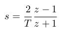
The effect of "frequency warping" is taken into account in the filter design.