Example 5
The procedure for creating a motion diagram is illustrated in this simple example.
The task:
The following slave motion is to be implemented for a rotation of the master axes from 0 to 360 degrees.
- A rest (stationary slave axis) between 0 and 20 degrees
- A turn at 180 degrees and 240 degrees at slave position 100 mm
- A rest (stationary slave axis) between 340 and 360 degrees
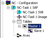
In a new configuration of the System Manager, we use a right mouse click under NC Configuration to insert a new task under a Append Task. In the Tables that it contains, we right click with the mouse to create a new master using Append Table, and also to create a slave under Append Slave.

When Slave 1 has been selected in the tree, both the Graphic and Table Window appear.
The Insert Point command is used in the graphic window to click the points at their approximate positions in the window. The corresponding values will then be inserted into the table window.
A certain amount of information must be added so that this motion plan can become a motion diagram. For the first and fourth sections we use the Synchronous Function command to specify by clicking with the mouse in the corresponding sections that a linear motion should take place there. In the second section in the table of Function the AccTrapezoid_RT is selected and in the third one the the AccTrapezoid_TR.
The position of the points can now be manipulated using the shifting commands.
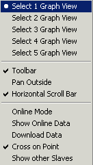
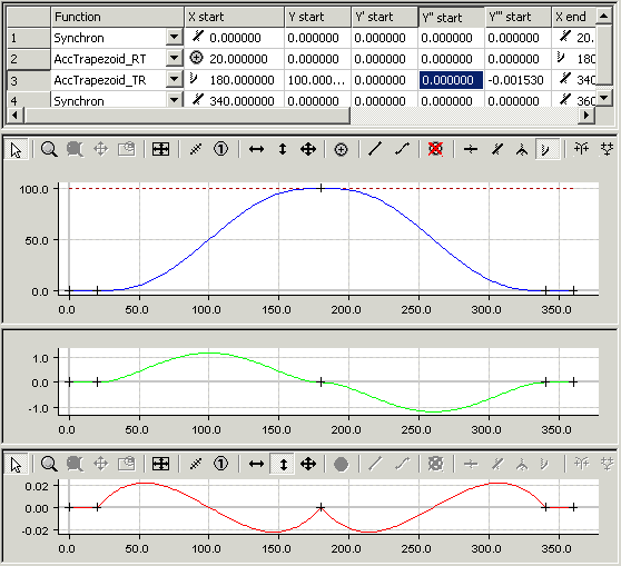
If Select 3 Graph View is selected with a right mouse click, then in addition to the position of the slave in the first graphic window, the velocity is shown in a second window and the acceleration in a third.

The size of the windows can be altered interactively, by placing the mouse on the edge and dragging it with the left mouse button.
So that the positions can be reached exactly, they are entered in the table view.

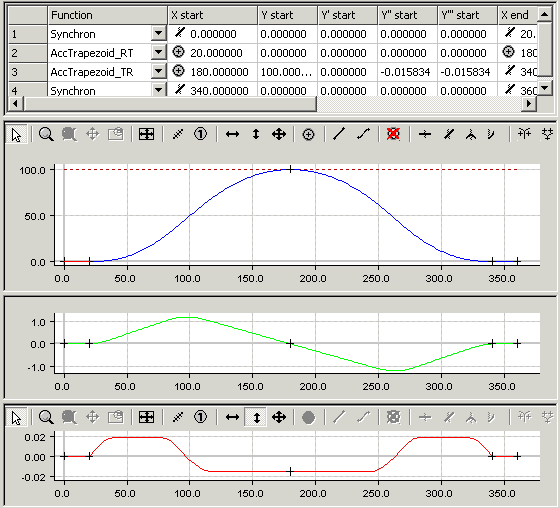
The boundary values at the point (180,100) are yet that the acceleration is zero. Therefore the graphics looks like the former one. Because the AccTrapezoid can not fit to these boundary conditions the Polynomial of 5th degree is used. When the acceleration is modified from a certain value on the AccTrapezoid is used. Now one can fit in the graphics the acceleration to the needs.
