Method 1: characteristic a(n) in a polynomial or hyperbolic form
In the range above the limit speed, the current acceleration is optionally specified via a third-degree polynomial or via a hyperbole function. In the case of both characteristics, a constant acceleration aconst is used in the range below nlimit. This corresponds to the acceleration at nominal speed. The characteristics apply to both the speed setup and slowdown phases.
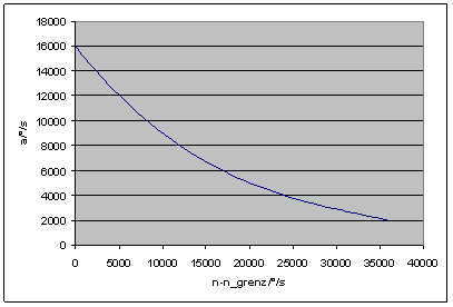
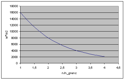
 Fig.14: Course of acceleration in accordance with a polynomial or hyperbole
Interpolation points on the drive characteristic a(n) are used to determine the coefficients of the characteristics. Four or three interpolation points are needed to determine them.
One interpolation point P1=(n1, (a(n1)) is already defined by the parameter for constant acceleration aconst and the limit speed nlimit, and the user can define the remaining three or two along the drive characteristic a(n). It is best for the abscissa values to be at a constant distance. The equations for determining the coefficients are listed below.

Polynomial

Example of determining characteristics
Interpolation point | Acceleration a [°/s] 2 | Speed n [°/s] |
|---|---|---|
1 | 16000 | 12000 |
2 | 8000 | 24000 |
3 | 4000 | 36000 |
4 | 2000 | 48000 |
a_const = 16000[degrees/s2] to nlimi = 12000 [degrees/s]
We arrive at the following for the coefficients:
b3 = -1.92901234E-10 [s/°2]b2 = 2.08333333E-5 [1/°]b1 = -0.88888888 [1/s]b0 = a_konst = 16000 [°/s2]As from the nominal speed (nlimit) the characteristic profile is as follows: n-n_limit/°/s

Hyperbole

Example of determining characteristics
Interpolation point | Acceleration a [°/s] 2 | Speed n [°/s] |
|---|---|---|
1 | 16000 | 12000 |
2 | 8000 | 24000 |
3 | 4000 | 36000 |
a_const = 16000[degrees/s2] to nlimit = 12000 [degrees/s]
We arrive at the following for the coefficients:
b2 = 4.166666E-1[]
b3 = 2.857142E-2[]
b1 = 2.285714E4[°/s2]
As from the nominal speed (nlimit) the characteristic profile is as follows:n-n_limit

Parameters
P-AXIS-00202 | Characteristic type: 1 (hyperbole) or 2 (polynomial) |
P-AXIS-00130 | Limit speed nlimit |
P-AXIS-00007 | Constant acceleration aconst for n<nlimit |
P-AXIS-00010 | Minimum acceleration amin |
P-AXIS-00026 | Coefficient b1 |
P-AXIS-00027 | Coefficient b2 |
P-AXIS-00028 | Coefficient b3 |
Parameterization examples
#
beschl_kennlinie.typ 1 Hyperbole
beschl_kennlinie.a_min 1400 [ ° /s*s]
beschl_kennlinie.n_grenz 12000000 [10-3 ° /s]
beschl_kennlinie.a_konst 16000 [ ° /s*s]
beschl_kennlinie.b1 2.285714E4 [°/s*s]
beschl_kennlinie.b2 4.166666E-1 []
beschl_kennlinie.b3 -2.857142E-2 []
#
#
beschl_kennlinie.typ 2 Polynomial
beschl_kennlinie.a_min 2000 [ ° /s*s]
beschl_kennlinie.n_grenz 12000000 [10-3 ° /s]
beschl_kennlinie.a_konst 16000 [ ° /s*s]
beschl_kennlinie.b1 -0.88888888 [1/s]
beschl_kennlinie.b2 2.08333333E-5 [1/Grad
beschl_kennlinie.b3 -1.92901234E-10 [s/Grad²]
#