Notes on analog aspects ‑ dynamic signals
This chapter deals with the problem of measurement/acquisition of actual analog electrical signals from the industrial automation environment. Such signals are generated by sensors and measured by automation components. With this information, the (software-based) control system perceives the physical system reality and derives follow-up actions from it.
The signals are formed electrically and measured analogously as
- signals via industrial interfaces 10 V, 20 mA, …
- signals from the sensor directly: voltage of a battery [V], bridge signal [mV/V], current measurement [A], resistance [Ω]…
Signals that do not have to be measured electrically but are already present virtually in the control system can also be analyzed with the tools listed below but are not the focus of this document.
Introduction
This chapter deals with the usual "circumstances" of real analog sensor signals in industrial environments, which are considered "over time", in the course of which information is transmitted to the controller in the form of
- amplitude or signal level, or "signal is present", "signal is not present"
- frequency or
- a mixture thereof
In practical terms and based on actual examples, this means
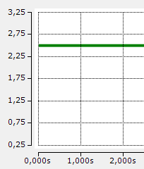
- the signals are "constant" → battery measurement (but only without load)
- or are constantly changing, unpredictable, e.g.:
(continuous weighing process)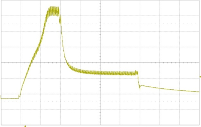
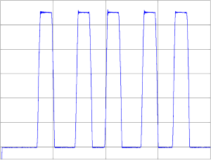
(excitation of a solenoid valve) - In most cases they are not constantly cyclic "deterministic", like a 1 kHz sine wave from a frequency generator, but have pauses and change their frequency, i.e. they are "stochastic", e.g.:
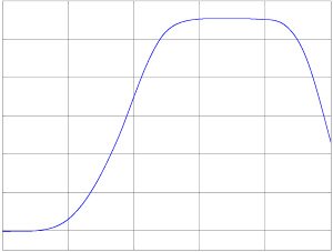
(excitation of a solenoid valve) - Sometimes they are very steep-edged:
- Or not:
- They are never "ideal" but are subject to disturbance, interference and attenuation:
- They can be superimposed, apparently consisting of two superimposed sine signals:
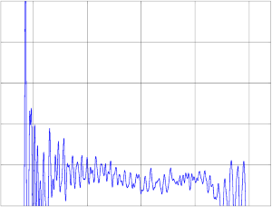
- If many frequencies are involved, this is indeed the case:
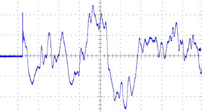
(the beginning of a song, measured at the loudspeaker) - They change over time, temperature, humidity, installation position, etc.:
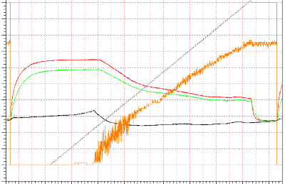
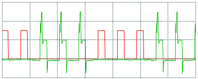
- And a desired square wave signal (green) quickly becomes something else (red) on the line:
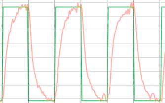
- Sometimes all these factors interact, in which case the question arises: "what is the measured value"?
- In any case, they rarely look as ideal and cyclical as here:
Notice | |
The time axis is relative In the above examples the x/time axis is intentionally not labeled. Whether a signal is fast/slow, flat/steep "only" depends on the evaluation against the set requirement and the measuring time: in a mechanical tensile test (tear test), the signal changes only slightly for a long time, until very steep signal changes in the µs range are suddenly observed at the break point |
Although "real" industrial signals are not permanently uniformly ideal and sinusoidal, it is helpful to use the terms and tools of theoretical signal analysis to characterize effects and test the effectiveness of measures. Keywords such as "signal frequency", "edge steepness", "attenuation" and similar can then be applied to the real signal section by section.
This chapter therefore considers the extensive theoretical basis of signal theory (which can be studied via www.wikipedia.com and standard text books) through the eyes of the industrial automation engineer and focuses on
- signal parameters µV..kV, corresponding to Ampere,
 etc.,
etc., - signal frequencies 0 Hz to ~1 MHz,
- non-constant signals,
- that are not ideal.
Practical applications
Analog devices can measure as follows, in order of increasing complexity:
- Static electrical variables that do not change over a "short" time: DC voltage or DC current, generally one constant variable, "DC" for short (direct current). This is available e.g. as output voltage of a battery that is not under load.
Note: "short" is a subjective term that very much depends on the particular situation - Dynamic electric variables that change over time: AC voltage or AC current, generally one alternating variable, "AC" for short (alternating current). It has a signal shape that repeats with a certain period. This is present, for example, in the German power supply system with a sinusoidal signal form of 50 Hz or appears in the form of "rapidly" changing measured variables on machines. The reciprocal value of the period value is the frequency f; unit Hz. The maximum value is called amplitude among other things and can refer to the current or voltage value. For a first approach it can be regarded as a constantly repeating, periodic/deterministic signal.
- Mixed signals: These are a "mixed form" of several overlaid alternating variables. They take the form of a voltage or current signal containing several alternating variables with different frequencies and amplitudes, and may also contain a DC voltage, which is usually referred to as the "DC component" or "offset". Here too, the first approach should be based on constantly repeating, periodic/deterministic signals
- If the signals change in their frequency/amplitude, so-called non-deterministic/stochastic (random) signals, we finally encounter the real cable reality.
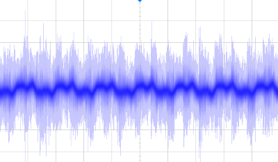
A particularly good example of a signal of this kind would be a "noise signal".
It should be noted that the "actual" signals that appear – the "real" signals – are more or less mixed signals, because electronic components are always "lossy" and usually distort a "pure" signal shape. Ideal signals are theoretical variables where no losses are taken into account. Therefore, a signal is specified as a real occurring mixed signal among other things by its maximum amplitude A and the lowest frequency that it contains, i.e. the base frequency.
In addition, the constancy of a frequency in real environments is usually not possible either due to physical conditions. As a rule, it is rather complicated to create an oscillation generating system that is subject to virtually no changes of frequency over time.
Below, we explain what fundamentally needs to be observed when measuring dynamic signals with analog devices.
Signal theory
The basic accuracies specified in the Beckhoff IO documentation apply in general to static (DC) signals unless stated otherwise. When determining the specification, a DC signal is applied and a measurement is only carried out when the entire measuring system has completely settled down and the measured value does not change within a "short" time. At attempt is made in the production calibration to minimize the residual deviation ∆GDC.
On account of the losses and inertia of resistors, inductances and capacitances in the amplifiers of an electrical input circuit as well as the finite calculation times of digital signal processing blocks, settling requires a certain time (also referred to as settling time). Depending on the layout, this can take between a few nanoseconds and several seconds. Side note: If the thermal settling of the devices/cables also has to be taken into account, it can even take many minutes.
If, on the other hand, a dynamic, time-dependent (AC) signal is measured, the measuring system can never settle to a completely stationary state, because the signal is constantly changing and the rate of change of the AC signal is greater than the settling time of the system. This gives rise to an additional frequency-dependent deviation that is not covered by the DC specification ∆GDC. For example, if the dynamic signal is a sine wave
S(t)=A∙sin(2∙fSignal∙f∙t),with amplitude A, the additional deviation can be displayed as gain deviation ∆GAC. In reality, this means that Ameasured ≠ Asignal, where not only attenuation Ameasured < Asignal is possible, but also inadvertently amplification Ameasured > Asignal. The total gain deviation then results in
∆Gtot = ∆GAC + ∆GDC (frequency-dependent)
where ∆GAC is the additional gain deviation due to the alternating signal.
Below, a real signal is examined whose signal composition (base frequency, noise, overlaid interferences) changes constantly; nevertheless, an ideal case is assumed with regard to its frequency, which is then constant (f = const.).
Note: since this method has its historical basis in signal transmission in the AC range, the corresponding terms are used: gain/amplification, dB, attenuation and so on. As described later, this often leads to common statements in logarithmic [dB] representation, which have to be converted for low-frequency [ppm] assessment.
The frequency response in dB and ppm
This frequency-dependent deviation can be represented as a so-called frequency response. The frequency response describes the ratio of the output signal to the input signal with regard to the amplitude and the phase for a certain frequency range.
The phase shift is irrelevant in many applications and is therefore often not displayed. However, it should be borne in mind that not only the amplitude of the output signal can change over the frequency, but also the phase of the output signal relative to the input signal.
On a graph of the frequency response, the x-axis always represents the frequency fsignal. The amplitude ratio is displayed either linearly or logarithmically (preferably in the unit dB [decibel]) in the y-axis. Depending on the analysis objective, the linear or logarithmic scaling shows certain characteristics better. It should be emphasized that the scaling (linear/logarithmic) is independent of the unit (Hz, ppm, dB)!
Scaling variants | x axis / frequency | ||
Linear [Hz] | Logarithmic (then preferably in [dB] ) | ||
y axis | Linear | Helpful for accuracy considerations in the ppm range | Unusual, with increasing frequency attenuation is no longer clearly shown
|
Logarithmic (then preferably as attenuation in [dB] ) | Not very helpful the lower frequency range is poorly resolved | Usual for dB representation
| |
The unit dB (decibel, 1/10 Bel) is used to describe the ratios of two values to each other. It has no unit itself! A dB is defined for two powers P1 and P2 by the following equation
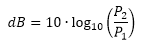
With this representation method, for example, it is possible in a system chain with amplifying and attenuating elements to determine a total value simply by the addition and subtraction of the individual values instead of multiplication and division.
For the two electrical power values on the same resistance, the general equation P = U · I, together with Ohm's law, produces a square ratio for the two currents I1 and I2 as well as for the two voltages U1 and U2:
|
|
|


transferred to the ratio of the two powers P1 and P2:
|
|
|


The square can be written before the logarithm and the following equation thus results in general for two amplitudes A1 and A2 as field variables:
In this context it is helpful to note the following conversions of dB and amplitude ratios:
[dB] | [A2/A1] |
|---|---|
40 | 100 |
20 | 10 |
3 | 1.414 |
0 | 1 |
-3 | 0.707 |
-20 | 0.1 |
-40 | 0.01 |
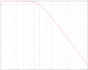
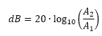
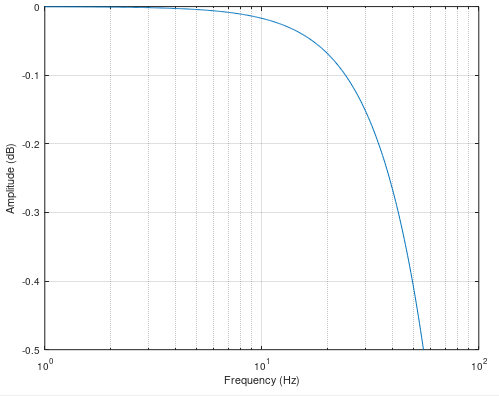
The following illustration shows the double logarithmic amplitude response of an "ideal", i.e. "calculated" RC circuit configured as a low-pass filter, where R = 1 MΩ and C = 1 nF. Both amplitude and frequency are represented logarithmically:
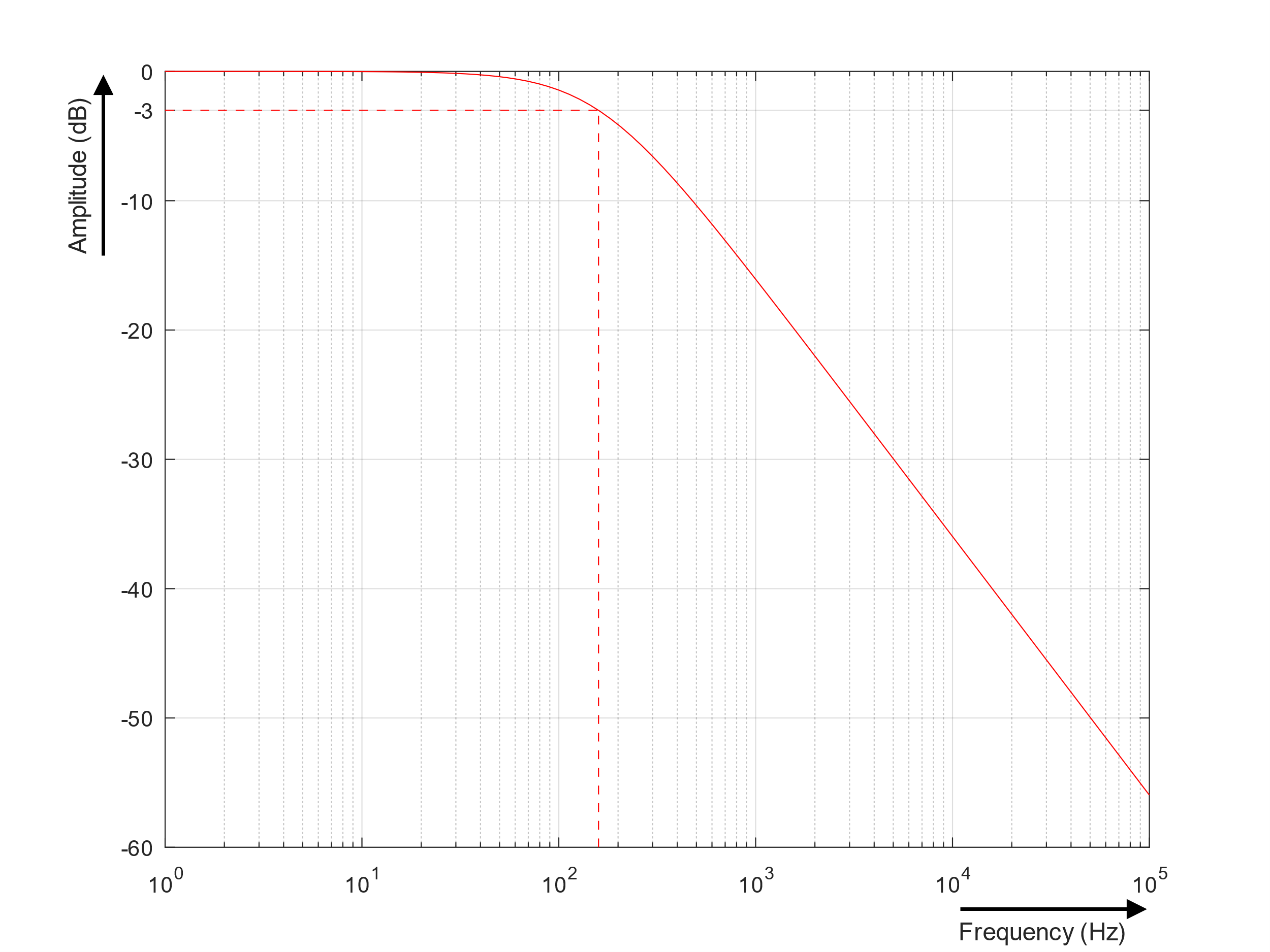 Fig.44: Amplitude response of a low pass RC circuit
The input signal passes through almost without attenuation up to the frequency marked by the dotted line (fsignal ≈ 159 Hz, amplitude at ‑3 dB, 102 = 100!). Above = to the right of this frequency (obviously even a little before that), the circuit begins to attenuate the input signal noticeably. The marked frequency obviously separates two areas with different behaviors. It is therefore also referred to as the cut-off frequency fc.
Depending on the background to the problem, there are various parameters to describe the amplitude/frequency responses. The ‑3 dB point is one possible parameter and is often used with analog RC filters or digital Butterworth filters.
The graph gives the impression that the amplitude passes through entirely unattenuated up to f = 20 Hz, but that is not the case. Like a view from afar, the dB representation conceals the fact that, from a microscopic point of view with a resolution in % = 1/100 or ppm = 1/1000000 = 10‑6, attenuation does indeed take place. And this is particularly interesting when it comes to analog measurement modules that are specified with a basic accuracy in the ppm range.
The next illustration shows the same relative attenuation, but in ppm. It is a double-linear representation of the amplitude response of the RC circuit:
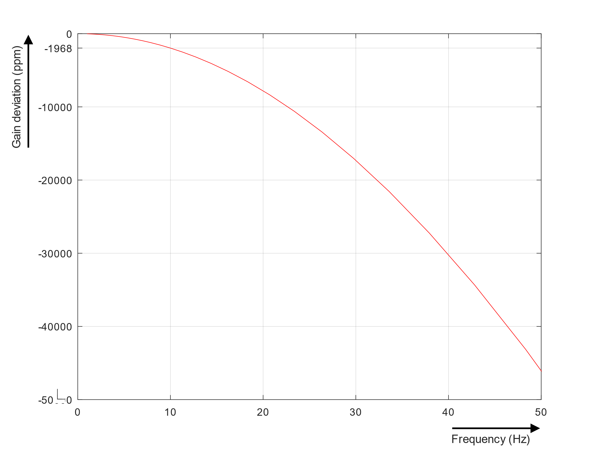 Fig.45: Relative "gain" deviation of the RC circuit in ppm up to 50 Hz
The graph shows that at 10 Hz the output amplitude is already smaller relative to the input amplitude by 1968 ppm - in fact a measurement error. Since it is known in concrete terms, this can even be called a measurement error.
From the above table, we therefore select the small attenuation range of interest for metrological devices with some example values:
dB vs. ppm | ||
|---|---|---|
[dB] | [%] | [ppm] |
-0.001 | 0.01 | 115 |
-0.005 | 0.06 | 575 |
-0.01 | 0.12 | 1151 |
-0.02 | 0.23 | 2300 |
-0.04 | 0.46 | 4595 |
-0.08 | 0.92 | 9168 |
-0.2 | 2.28 | 22763 |
-0.4 | 4.5 | 45007 |
-0.8 | 8.8 | 87989 |
-1.6 | 16.82 | 168236 |
-3 | 29.21 | 292054 |
An attenuation of ‑3 dB thus means almost 30%FSV or almost 300000 ppmFSV amplitude error! And measurement accuracy of 0.1% corresponds to about 0.01 dB. This sounds dramatic, and rightly so, and is lost in the usual logarithmic dB representation.
The "problem" of the dB representation, however, is mainly due to the fact that a dB representation usually extends over several Hz orders of magnitude - precisely in order to represent the high attenuations and to show linear behavior over wide frequency ranges.
When zooming into the dB representation and for consideration only lower frequency parts, the information is much better:
But before we look at the effect of the frequency response specifically on analog inputs, we need to look at other phenomena.
Filters are everywhere
The above-described "manipulation" of the frequency response takes place by means of so-called filters along the signal processing chain
- unavoidably in all electrical, i.e. analog elements
- manipulably in the digital, i.e. software elements
Filter can be subdivided according to their application and their implementation. On the one hand, filters are used to influence or change the signal in the time domain, for example to smooth signals or to remove the DC component. Frequency-selecting filters aim to separate certain frequency bands from one another. The above example with the RC circuit is a low-pass filter that allows low frequencies to pass through with almost no attenuation while strongly attenuating higher frequencies. In addition to low-pass filters there are other filter types, such as high-pass filter, band-pass filter and band-stop filter. Other user-defined filters can be designed for other applications that don't fit into these categories, or for complicated applications.
Filters can be constructed either as analog filters (active or passive) or as digital filters in software.
Filters are characterized by their response to certain signal types. Each linear filter has a pulse response or step response and a frequency and phase response. The step response describes the temporal amplitude curve when an (ideal) step is connected to the input; the frequency response describes the amplitude gain (or phase shift) between the output and input signal. If one of the three graphs is known, the other two graphs can be calculated from it.
With many filters, the -3 dB frequency indicates the signal frequency at which the signal is attenuated by -3 dB. As already indicated above, it is also referred to with certain filter types as a cut-off frequency, at which the output power has been halved and the amplitude has fallen to 1/√2 = approx. 70% in comparison with the input amplitude, corresponding to a attenuation of approx. 30%.
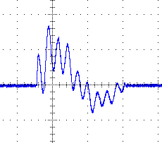
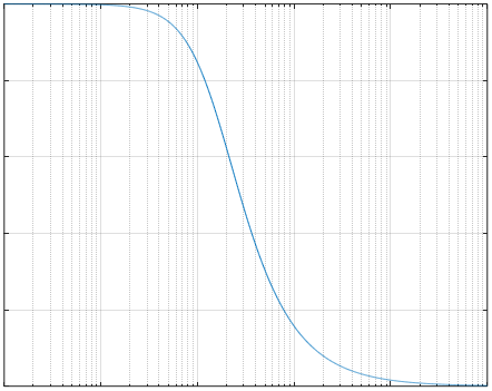
Digital filters can be divided into two categories: FIR filters (finite impulse response filters) and IIR filters (infinite impulse response filters). As the names suggest, the two filter types differ by their pulse response in the time range. The following illustrations show the differences in the pulse response of the two filter types:
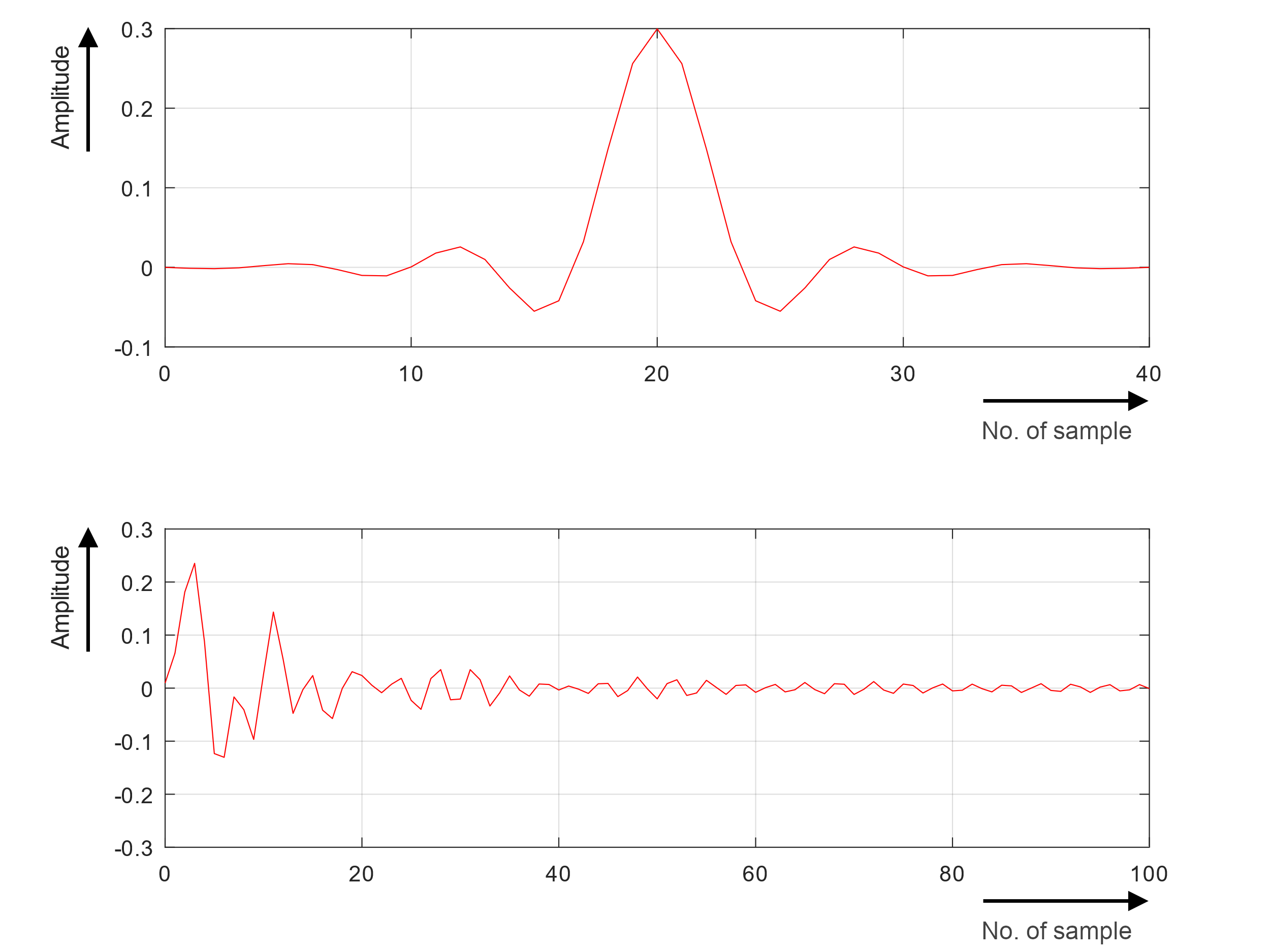 Fig.46: Example Impulse response of two filters; top FIR filter, bottom IIR filter
FIR filters are described by the mathematical equation
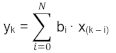
Only input data x(n‑k) are used which are accordingly sampled amplitude and time discrete values. With an FIR filter, the impulse response becomes zero after a finite time, which ultimately means that it is always stable, since there is no feedback, and can exhibit a linear phase response. However, FIR filters require a higher filter order to achieve a performance similar to IIR filters, which results in a longer calculation time. "Higher order" means that more filters have to be calculated one after the other.
IIR filters are described by the following equation
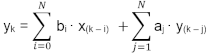
In order to calculate the output value y(n), the previously calculated output data y(n-k) are used in addition to the input data x(n-k). The filter is therefore recursive. For that reason, IIR filters are also called recursive filters. The pulse response of an IIR filter is infinite and thus never settle to zero stationary. This can ultimately lead to instability.
A fundamental effect was mentioned here by the way: the more effect/costly a digital filter is, the higher its complexity and thus the longer its calculation time in the software. This leads in practice to a signal delay.
Nyquist, Shannon and false signals: "Aliasing"
The fundamental sampling theorem states that, if a measuring device samples an analog signal at a constant (steady) sampling rate that is more than twice the highest frequency component present in the signal, the original analog signal can be fully restored from the discrete data points.
(Note: the highest frequency present in the signal is referred to as the bandwidth of this signal.)
After all, this is the actual aim of an analog measurement, i.e. the original signal should be available digitally as accurately as possible ("correct") and complete in the control system for further processing in the program. However, a limit must be imposed here that only signal components (frequency ranges are meant here) that are essential for the further process need to be detected. Ideally, the user will make a conscious choice and reflect this limitation. Example: A slow temperature control must be insensitive to low-frequency signals, because this could disturb the controller.
In order to record the analog signal as accurately as possible, the signal bandwidth fsignal must be limited through suitable filtering (see chapter on "Filters") so that only the desired signal but no interfering signals pass through, and the sampling rate fsampling must be selected such that the signal can be restored from the data points as a true representation of the original signal. We therefore have to examine the relationship between the actual sampling rate fsampling and fsignal.
(Note: each measurement takes place in the two dimensions time and measured variable. Here we concentrate on the temporal dimension, i.e. the sampling).
Theoretical considerations relating to the sampling theorem are illustrated with an analog signal and different sampling rates.
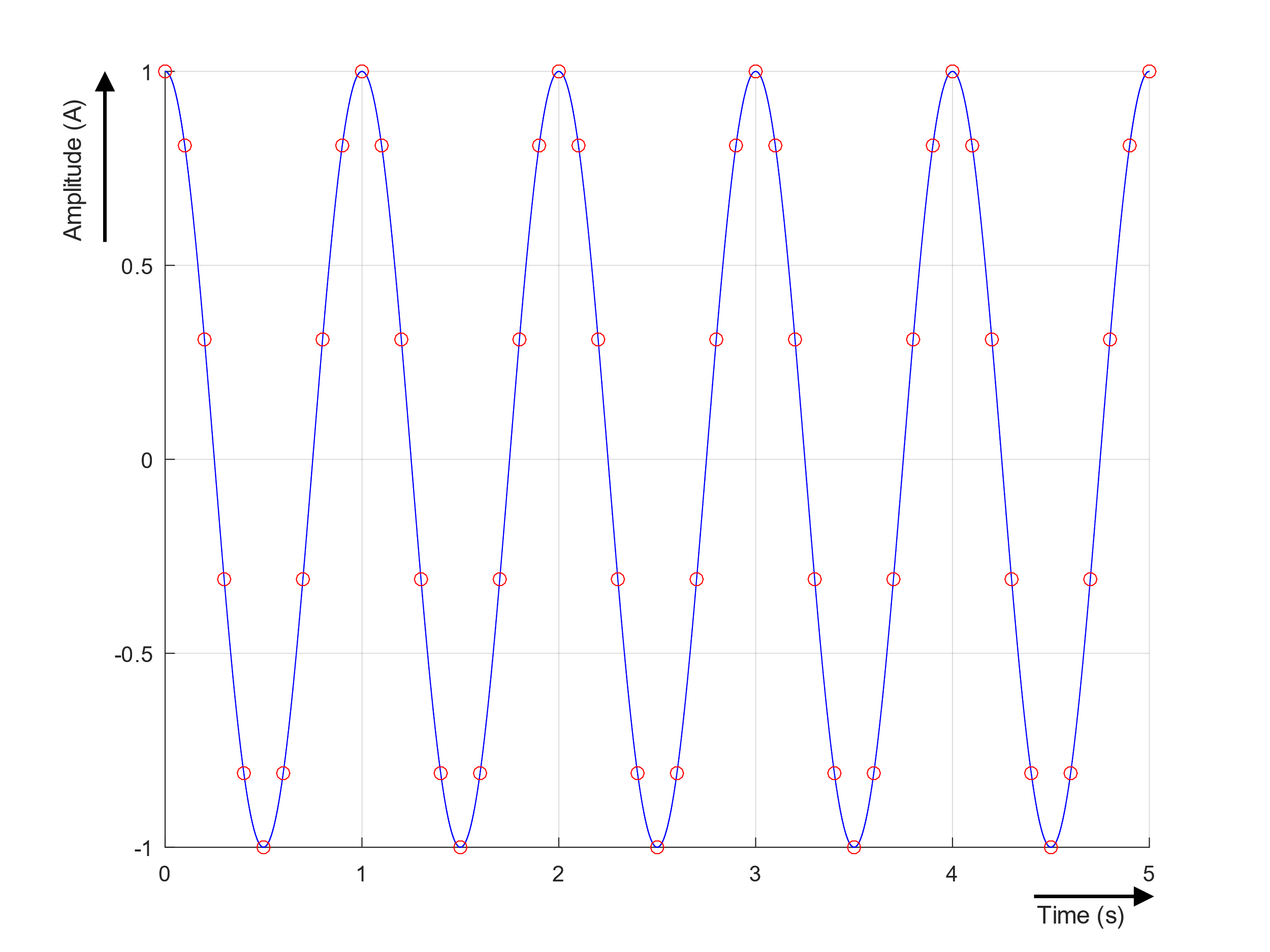 Fig.47: Analog signal (cos) with a frequency of 1 Hz (blue line) sampled at 10 Hz (red circles)
The analog signal with f = 1 Hz was sampled with fsampling = 10 Hz. The largest (and only) frequency component in this sample is 1 Hz, therefore fsignal = 1 Hz and fsampling = 10∙fsignal. It is easy to see that the original analog signal can be reconstructed from the discrete values. For example, a fast Fourier transform (FFT) could be calculated from the above data. This would easily be possible, and the resulting spectrum would extend to fsampling/2 = 5 Hz, with a resolution of 0.2 Hz.
If the analog signal had not been a "pure" sine wave but had been harmonically distorted and noisy, then fsignal would no longer be 1 Hz but usually much larger due to the higher frequency components contained in it. In this case the chosen fsampling must be significantly greater than f, depending on the evaluation aim. This also applies in general terms, as will be explained a little later.
The next figure shows what happens if the fSignal = 1 Hz signal is sampled at fsampling = 2 Hz, i.e. fsampling = 2 · fSignal.
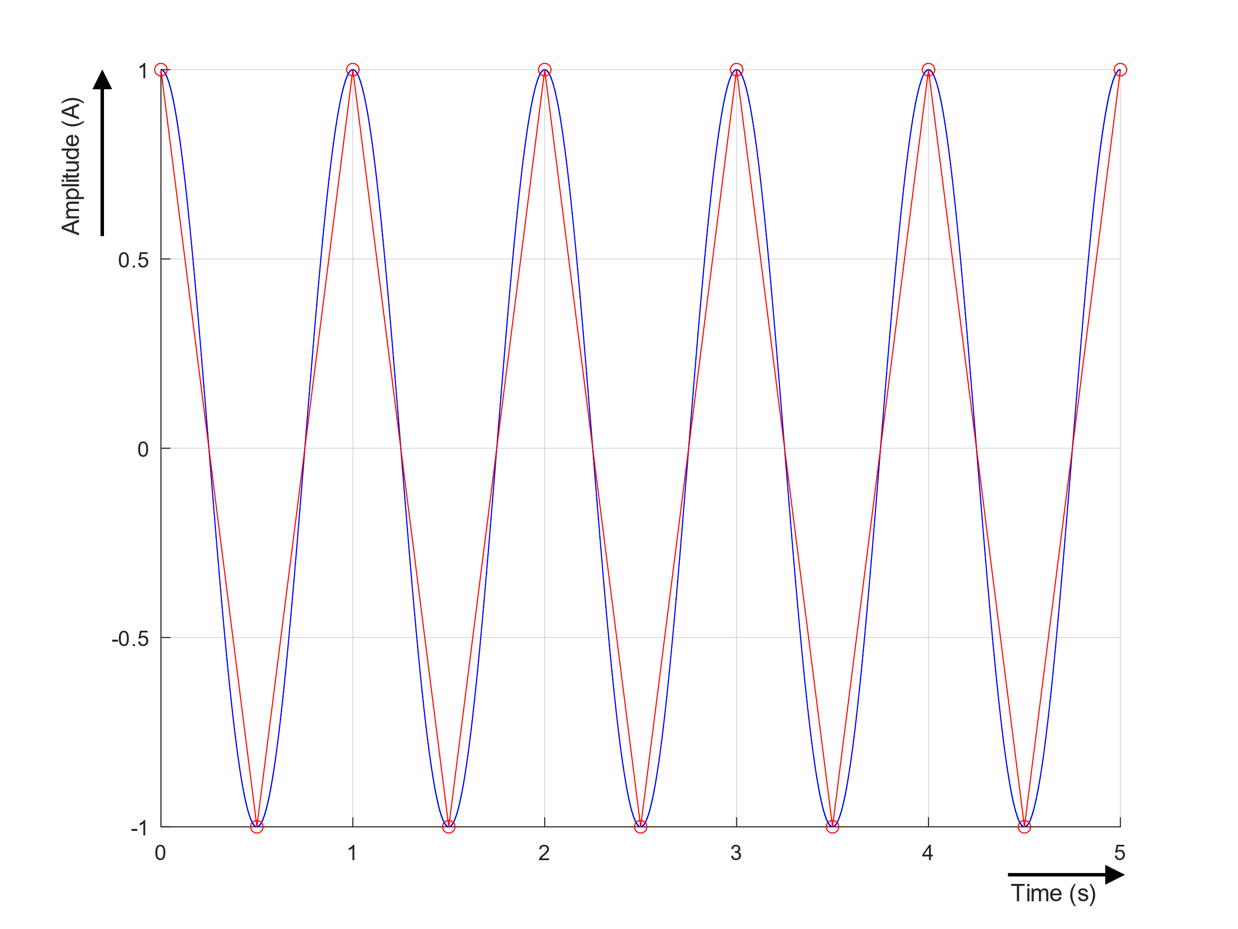 Fig.48: Analog signal (cos) with a frequency of 1 Hz (blue line), sampled at 2 Hz (red circles) and interpolated / "traced" (red line)
Since in this sample a specification resulting from the sampling theorem is just about met, it is still possible to detect the frequency and amplitude of the signal: fsampling is equal to 2 ∙ fSignal.
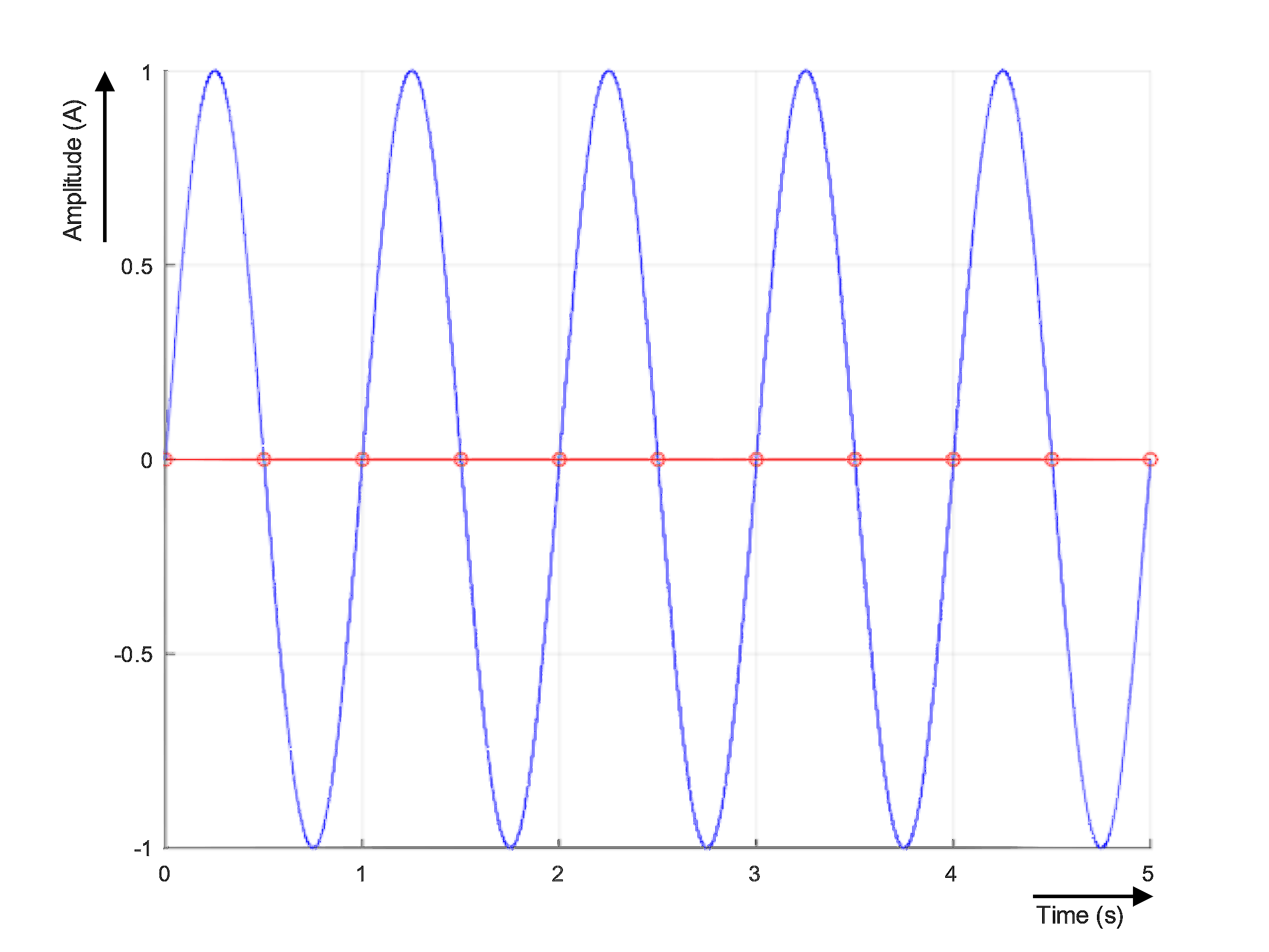
However, this is no longer possible in general, as the following problem becomes apparent here, if one imagines that the sampling moments would be randomly shifted by 90° relative to the signal. In this case the value of the signal at each sample point would be zero, and it would no longer be possible to detect the frequency or amplitude.
In practice, it is much more likely that the measuring points lie "somewhere" on the signal:
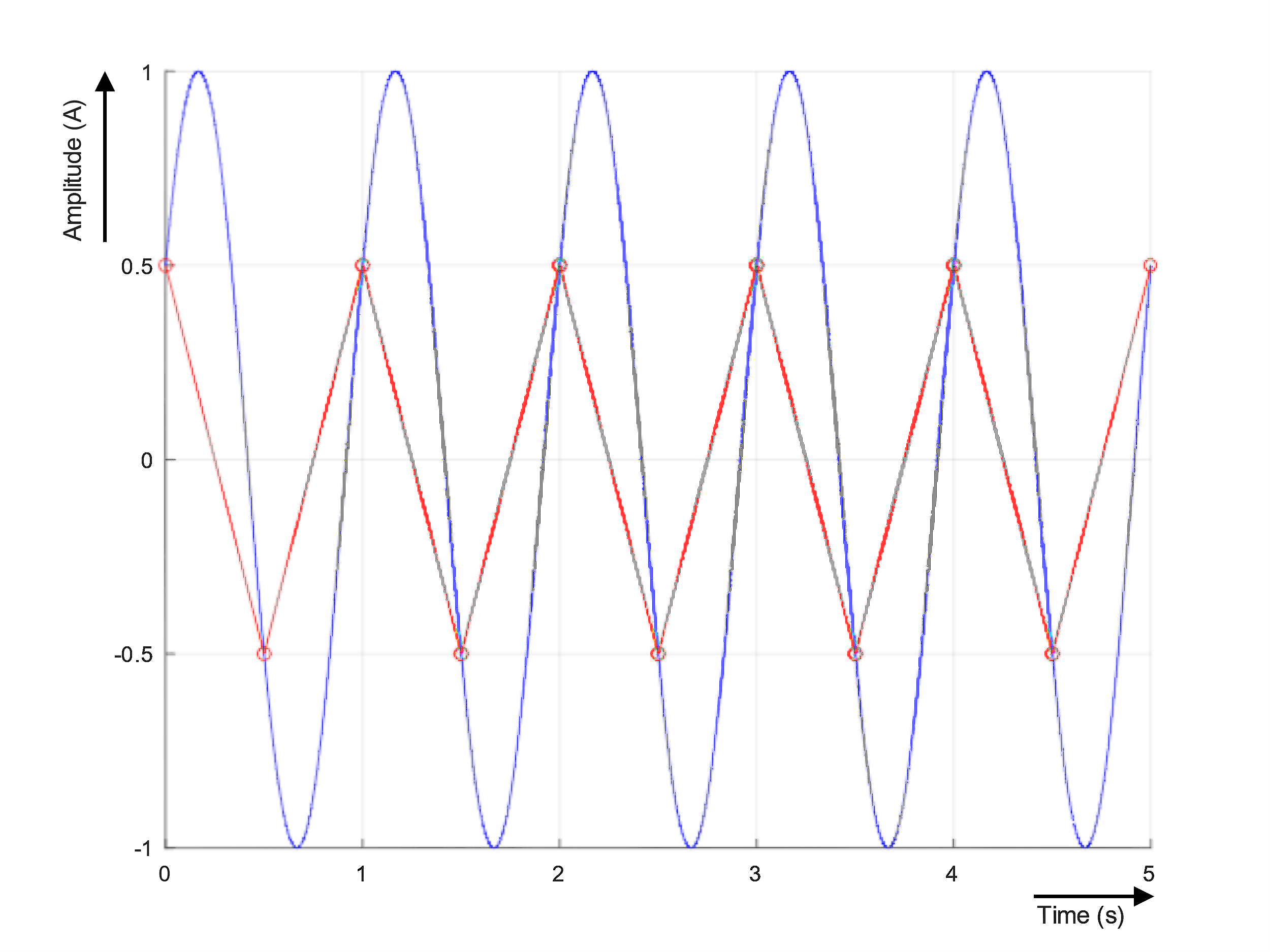
In this case, at least the frequency can still be determined due to the zero crossings, but the peak value (and thus very important signal information) cannot be determined because it is not clear where the measuring points are located on the original signal. In practice, however, neither fsampling nor fsignal will be highly constant, and longer observation will result in variable phasing and the peak value will still be caught "at some point". However, this is of little use with fast-moving industrial signals.
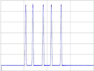
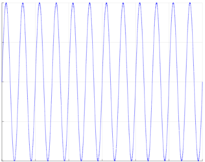
After these theoretical considerations, let us now look at a concrete real example: the induced voltage of a rotating gear wheel on a coil as speed sensor results in the following representation in TwinCAT ScopeView:
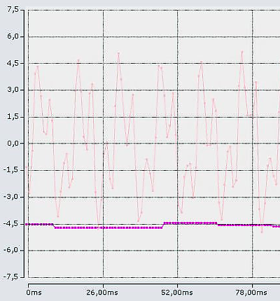
Selecting a higher sampling frequency (sampling rate) would be advantageous here in order to be able to follow the amplitude curve better, because signals seem to overlap here. The zero crossings may be sufficient for speed observation.
The frequency

is also called the Nyquist frequency. If an analog signal contains frequency components equal to or greater than the Nyquist frequency, the original signal can no longer be reconstructed. In practice, the Nyquist frequency is selected to be at least a factor of two to three times greater than the bandwidth of the signal frequency fsignal.
The resulting problem of the non-reconstructable original signal due to fsignal ≥ fNyquist was already hinted at in the previous example. The figure below illustrates the problem.
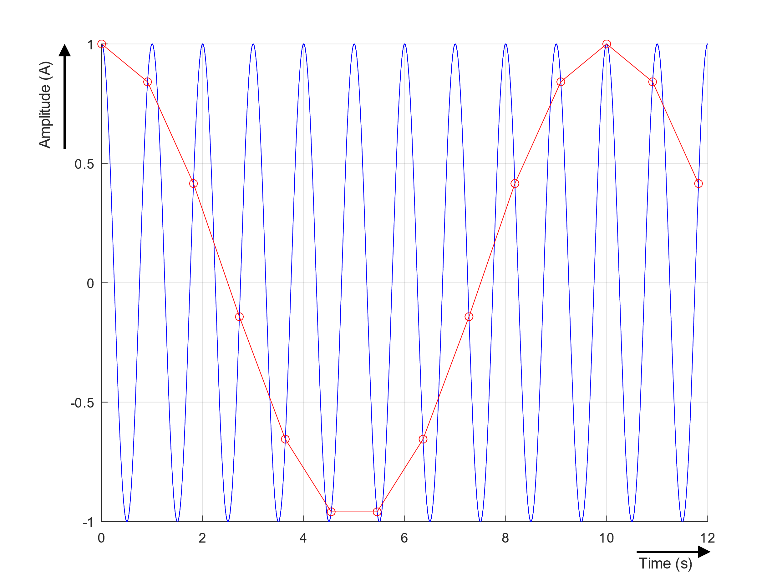 Fig.49: Analog signal (cos) with a frequency of 1 Hz (blue line), sampled at 1.1 Hz (red circles) and interpolated / "traced" (red line)
Here fsampling = 1.1 · fSignal. The frequency information of the original blue signal has been lost. From the control system point of view (which only "sees" the red measuring points), it appears that the measured red signal is a signal with a lower frequency. This effect is called aliasing because a different frequency is detected. It is a common problem when the fundamental sampling theorem (also called the Shannon-Nyquist sampling theorem) is violated. The apparently detected alias frequency in this case is falias = 0.1 Hz.
The Shannon-Nyquist theorem and alias effects focus solely on the question of whether the original analog signal can be reconstructed from the sampled values. This cannot be the sole criterion for selecting an analog input, but it is an essential one. In practice, there are situations where the sampling theorem is deliberately violated, e.g. in order to reliably detect fast signal changes. Since the user already knows a lot about the analog signal to be measured, such considerations are quite possible and in many cases help to optimize the measuring system.
Further effects
Further phenomena from the field of measurement of alternating variables such as noise, distortion, signal cross-talk and signal delay in detail will be further illuminated here in due time.
Reaction or recording? Or both?
Finally, from an application perspective, it is important to consider whether the application is a response task, a data recording task, or a mixture of both.
- Reaction:
- Example: a distance sensor with a 10 V analog output detects an object approaching on a conveyor belt at 10 m/s and, if 5 V is exceeded, a valve for a paint application should be opened in the shortest possible time. Another extreme example would be current control in a software-controlled magnetic bearing.
- The following would need to be selected:
# an analog input with high sampling rate, open filter, possibly even DistributedClock timestamp function (although the reference to the absolute world time probably does not matter)
# short EtherCAT cycle time and short PLC cycle time, if necessary 100 µs or less - Analog accuracy is secondary here; a long-term recording of the measured values will probably not be carried out either
- Data recording
- Example: a strain test lasting several days on a steel structure with slow movements in the seconds range.
- The following would need to be selected:
# a precision analog input; important here are low noise and high temperature insensitivity, synchronization across multiple channels, possibly even absolute time synchronization to the GPS clock
# slow EtherCAT cycle time, the analysis program in C/PLC/MATLAB® will probably demand quite a lot of the controller - The sampling rate is probably secondary here. Signals with short rise and fall times as well as attenuation issues due to high frequencies are not expected
- In addition to the above extreme examples, most industrial applications are a mixed form of the two. That said, only the user can judge whether a reaction in the 100 µs range is "fast" in view of his problem: for temperature monitoring in the seconds range, this is "too fast", for laser monitoring "too slow".
At the end of the day, therefore, the analog and temporal characteristics of the Beckhoff analog devices have to be judged against the problem.
Effect on analog input devices and the design of the same
Depending on the intended application objective, some basic decisions have to be made by the manufacturer of analog inputs during the design phase. The different answers to the questions
- Attenuation: at what frequency does attenuation occur, how does it proceed?
- Sampling rate: which signal frequency should be measured at all, and with what accuracy?
- Delay: with what delay may the signal arrive in the controller?
have also been formulated at Beckhoff in the form of analog input devices. The user can find the right device for his application with the help of
- the Beckhoff documents (e.g. this manual)
- Beckhoff Sales
- and if necessary practical
tests.
Notice | |
kHz vs. kSps Note: in order to avoid linguistic misunderstandings in documentation and sales meetings, the incoming signal frequency fsignal is described at Beckhoff with the unit [Hz], and the technical sampling rate fsampling of the analog input with (samples per second) or [kSps] (kilo samples per second). |
Here is a rough classification for this:
- The EL30xx class with its 10 V/20 mA inputs is designed for simple measurements on slow signals with 12-bit resolution. Therefore, the hardware filter and the sampling rate are set very low.
- The EL31xx class (also: EP31xx, EJ31xx) with its 10 V/20 mA inputs with 16-bit resolution is designed for fast signals and reaction tasks. In order to promptly inform the controller of fast-changing signals, even the hardware filter is purposely selected higher than the sampling rate. However, this can lead to alias signals in measuring applications.
- The product group measurement technology of the ELM3xxx class (and: EPP35xx) are consistently designed for signal correctness in recording applications; the hardware filter lies well below half the sampling rate with its -3 dB point. The ELM3x0x class "10 ksps" is more suitable for faster tasks, while the ELM3x4x class "1ksps" is more suitable for slower tasks.
Moreover, key data that are suitable for the application area have been specially defined in the various special function terminals, which cannot all be listed here in detail. For example, the EL3632 / EPP3632 has variable hardware filters that can be adapted to the sampling rate.