Sources of error/disturbance variables
Inherent electrical noise of the load cell
Electrical conductors exhibit so‑called thermal noise (thermal/Johnson noise), which is caused by irregular temperature‑dependent movements of the electrons in the conductor material. The resolution of the bridge signal is already limited by this physical effect. The rms value en of the noise voltage can be calculated by:

In the case of a load cell with R0 = 350 Ω at an ambient temperature T = 20 °C ( = 293K) and a bandwidth of the measuring transducer of 50 Hz (and Boltzmann constant k = 1.38 · 10‑23 J/K), the rms en = 16.8 nV. The peak‑peak noise epp is thus approx. epp ≈ 6.6 · en = 111 nV (thermal noise, 99.9 % interval of standard deviation).
Example:
For a bridge with 2 mV/V nominal characteristic value and supply of UExc = 5 V, this results in an output voltage UBridge_max = 5 V · 2 mV/V = 10 mV (for the nominal load) and therefore a maximum resolution of 10 mV / 111 nV = 90090 digits. Converted into bit resolution: ln(90090)/ln(2) ≈ 16 bits. Interpretation: a higher digital measuring resolution than 16 bits is thus inappropriate for such an analog signal in the first step. If a higher measuring resolution is used, then additional measures may need to be taken in the evaluation chain in order to gain a higher information content from the user- and noise superposition, e.g. hardware low‑pass filter or software algorithms.
This resolution applies alone to the measuring bridge without any further interferences. The resolution of the measuring signal can be meaningful increased by reducing the bandwidth of the measuring unit.
If the strain gauge is glued to a carrier (load cell) and wired up, both external electrical disturbances (e.g. thermovoltage at connection points) and mechanical vibrations in the vicinity (machines, drives, transformers and audible 50 Hz vibration due to magnetostriction etc.) can additionally impair the result of measurement.
Creep
Under a constant load, spring materials can further deform in the load direction. This process is reversible, but it generates a slowly changing measured value during the static measurement. In an ideal case the error can be compensated by constructive measures (geometry, adhesives).
Hysteresis
If even elongation and compression of the load cell take place, then the output voltage does not follow exactly the same curve, since the deformation of the strain gauge and the carrier runs different due to the adhesive and its layer thickness.
Temperature drift (inherent heating, ambient temperature)
Relatively large currents can flow in strain gauge applications. A full bridge with four 350 Ω resistors for example has a current consumption of I = UExc/R0 = 10 V / 350 Ω ≈ 28.6 mA. The power dissipation of the whole full bridge is thus PExc = U · I = 10 V · 28.6 mA = 286 mW. Depending on application (a cooling of the strain gauge takes place by heat dissipation into the carrier material) and carrier material a not insignificant error can arise that is termed apparent elongation. Therefore, the strain gauges on the sensor material are often counter‑compensated by the manufacturer.
Inadequate circuit technology
As already shown, a full bridge may be able (due to the system) to fully compensate hysteresis, creep and temperature drift. Wiring‑related measuring errors are avoided by the 6‑conductor connection.
Measuring body and natural frequency
In the dynamic measurement of forces and weights, the setup and some of the properties of the transducer play an essential part in the attainable dynamics. The natural frequency of the complete system limits the dynamics of the application and is influenced by the spring constant of the measuring body and the coupled mass. The softer the measuring body ( = larger deformation under nominal load), the lower the natural frequency. In the case of measuring transducers with rigid measuring bodies, too, the coupled mass must always be included if the natural frequency is to be determined.
Load cells are technologically similar to force transducers, but have a softer structure and are usually manufactured at optimized cost. Consequently, the recommendation for the mechanical setup is:
- use a rigid measuring transducer and the lightest possible mounted parts,
- the natural frequency of the system should be at least 2‑5 times higher than the measuring signal frequency (i.e. the dynamically moved test specimen from the application that is to be measured),
- Natural frequency specifications in data sheets apply only to the measuring transducer without mounted parts and are therefore not useable in the field. It is better to calculate with the nominal measuring path and masses of sensor plus mounted parts. The real natural frequency can be checked by means of a frequency analysis of the pulse response by FFT or manually by determining the period.
The natural frequency is to be calculated with:
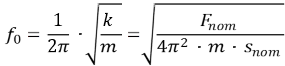 .
- f0 = natural frequency of the complete setup [Hz]
- Fnom = nominal force [N] or calculated nominal force by nominal load of the transducer [kg] and gravity of earth [m/s²]
- snom = nominal measuring path of the transducer (deformation under nominal load) [m]
- m = sum of dead weight and coupled mass [kg]
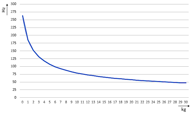
With Fnom = 450.5 N (50 kg nominal load and 9.81 m/s² gravity), snom = 0.18 mm, the resulting dependence on the mass, for example, is graphically: