2.5 D machining - Akima spline

In the following test program, a circle with a radius of 80 mm is approximated via 64 interpolation points. In the first run, the spline function is deactivated, and the linear blocks are interpolated. In the second run, the spline function is activated. The approach and departure travel blocks are programmed so that the tool entered the scanned ideal circular contour tangentially in each case.

%L uprg_secant 
N01 #SET ASPLINE MODE[2, 2] 
N01 P5 = 80 ( Radius ) 
N02 P3 = 64 ( Number of interpolation points ) 
N03 P4 = 360/P3 ( Angle staggering ) 
N04 G01 X-P5 F20 
N05 X0 
N06 G151 (Spline selection ) 
N07 $FOR P1=1, P3, 1 
N08 P2=P1*P4 F20 
N09 X=P5*SIN[P2] Y=P5*[1.0-COS[P2]] ( Calculation of secant interpolation points ) 
N10 $ENDFOR 
N11 G150 (Spline cancellation ) 
N12 XP5 
M29 
%L uprg_cir 
N01 P5 = 80 ( Radius ) 
N02 G01 X-P5 Y0 F20 
N03 X0 
N04 G03 JP5 
N05 G01 XP5 
M29 
%Main 
N100 LL uprg_secant 
N200 LL uprg_cir 
M30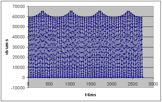

2.5 D machining - Akima spline 1: — Figure 1-28: Feed rate during interpolation of the secant contour (64 interpolation points)

The feed rate fluctuates relatively considerably because the non-linear slop function reduces the speed to 0 at the knee points of the linear blocks.

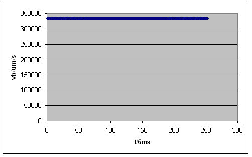2.5 D machining - Akima spline 2: — Figure 1-29: Feed rate during interpolation of the spline curves (64 interpolation points)

When the spline function is used, the interpolation time in the approximated circle drops for approximately 1/10 of the value of linear interpolation and the programmed feed rate is reached.