Example 2
The procedure for creating a motion diagram is illustrated again in this next simple example.
The task:
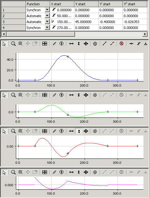
The following slave motion is to be implemented for a rotation of the master axes from 0 to 360 degrees.
- A rest (stationary slave axis) between 0 and 50 degrees.
- A velocity of -0.4 (normalized) at master position 150 and slave position 45.
- A rest (stationary slave axis) between 270 and 360 degrees.
- In the tree structure, create a master and its corresponding slave via MOTION > Tables (see Introduction).
- After selecting Slave 1 in the tree structure, both the graphic window and the table window appear.
- In the graphic window, click the approximate positions of the points in the window using the Insert Point command.
The corresponding values will then be inserted into the table window.
- To turn the motion plan into a motion diagram, you now need to add some information.
- For the first and fourth sections, use the Synchronous Function command to define a linear motion by clicking in the corresponding sections. In the second and third sections, the Automatic Function command is used to implement automatic adaptation to the boundary conditions.
By right-clicking and selecting Select Graph 3 View, the velocity in the second graph window and the acceleration in the third graph window are displayed in addition to the slave position in the first graph window.
- Enter a velocity of -0.4 in the table.
The acceleration is set to a zero value by default. Since at this point, however, no zero crossing of the acceleration is to be forced, but the jerk-free possible course is to be realized, the third point must now be moved interactively in the acceleration window in vertical direction.
- If you want to control the jerk, you can display the jerk by right-clicking and selecting Select Graph 4 View.
The motion diagram that has been created can be saved as a file in the slave's properties window.