Linearization
Problems can arise in association with a non-linear controlled system, in that a linear controller design based on this non-linear controlled system is found to be inadequate, because the controller can only be set up to operate optimally over one part of its working area.
The consequence is a loss in the control quality in many applications, or even that the control behavior is unacceptable.
The purpose of the curve linearization module presented here is to facilitate continued use of the familiar and proven procedure for designing linear control loops, but to improve the control quality.
The superposition of a characteristic curve module compensates for the non-linearity of the control system, resulting in approximately linear behavior.
This procedure is illustrated in the following functional diagram.
The curve employed in this procedure must describe the inverse of the transmission behavior of the particular combination of valve and hydraulic cylinder being used as exactly as possible; the net result of the inclusion of this characteristic curve module in series with the physically existing controlled system then results in an approximation to a linear curve.
 | Make sure the characteristic curve is as exact as possible in the knees. These points are particularly critical with regard to the linearization. |
The following functional diagram illustrates the use of the characteristic curve linearization to the TwinCAT axis control loop:
The curve required for the linearization process can be created and edited with the Valve Diagram Editor. After the curve has been created and loaded into the real-time environment, it can be activated within the axis control loop. This takes place in the Solution Explorer on the Analog tab of the drive or in general by ADS command.
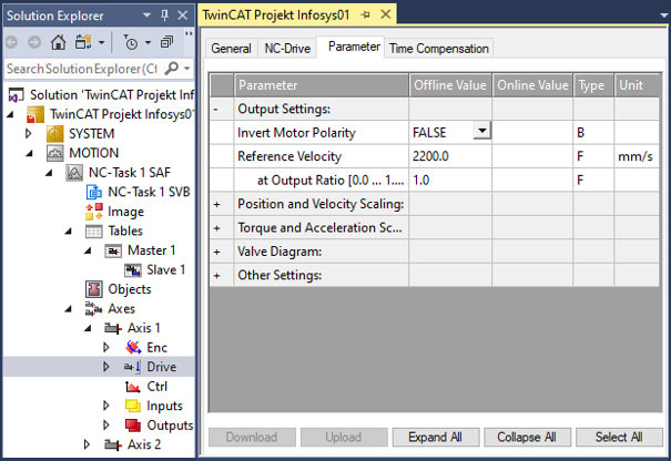
The unique table ID of the valve characteristic curve must be entered in the row "Valve characteristic curve: Id of the valve characteristic curve". You can choose between the types "Linear" and "Spline" in the row "Valve characteristic curve: interpolation type". (A table with equidistant reference points is created in the real-time environment, and this is interpolated at runtime using either a linear or a spline function.)
It is also possible to insert an output offset before and after the characteristic curve module.
The parameter "Drift compensation (DAC offset)" operates in the signal flow before the characteristic curve. An offset correction in the form of a velocity (in mm/s, for instance) can be added here.
An offset can be inserted in the signal flow after the characteristic curve with the parameter "Valve characteristic curve output offset [-1.0 ... 1.0]". At this point in the signal flow the offset is presented as a percentage value relative to the maximum output magnitude.
| Using the hydraulic characteristic curves The hydraulic characteristic curve can only be activated through entry of the table ID when
|
The parameters described on the drive's analog tab can also be specified by means of ADS commands (sent, for example, from the PLC).
Drive types:
The characteristic curve linearization described is supported by the following drive types:
- M2400 DAC 1 / DAC 2 / DAC 3 / DAC 4
- KL4XXX, EL4XXX, EL2521, IP2521/IP2512, KL2502_30K
- KL2531, KL2541
- Drive (universal)