Basic principles of strain gauge technology
 | General term: "device" This chapter is used in the documentation of several Beckhoff products. It is therefore written in general terms and uses the generic term "device" for the different device types such as terminal (EL/ELM/KL/ES series...), box (IP/EP/EPP series...), module (EJ/FM series…). |
Basic information on the technological field of strain gauges (SG)/ load cells as metrological instruments is to be given below. The information is of general nature; it is up to the user to check the extent to which it applies to his application.
- Strain gauges serve either to directly measure the static (0 to a few Hz) or dynamic (up to several kHz) elongations, compressions or torsions of a body by being directly fixed to it, or to measure various forces or movements as part of a sensor (e.g. load cells/force transducers, displacement sensor, vibration sensors). The evaluated quantity is the change of the strain gauge property (e.g. electrical resistance).
- In the case of the optical strain gauge (e.g. Bragg grating), an application of force causes a proportional change in the optical characteristics of a fiber used as a sensor. Light with a certain wavelength is fed into the sensor. Depending upon the deformation of the grating, which is laser‑cut into the sensor, due to the mechanical load, part of the light is reflected and evaluated using a suitable measuring transducer (interrogator).
The commonest principle in the industrial environment is the electrical strain gauge. There are many common terms for this type of sensor: load cell, weighbridge, etc.
Structure of electrical strain gauges
A strain gauge consists of a carrier material (e.g. a stretchable plastic film) with an applied metal film from which a structure of deformable thin film electrical resistor is worked in very different geometrical forms, depending on the requirements.
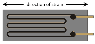 Fig.17: Schematic view of a strain gauge
This utilizes a behavior whereby, for example in the case of strain, the length of a metallic resistance network increases and its diameter decreases, as a result of which its electrical resistance increases measurable:
ΔR/R = k · ε.
ε = Δl/l thereby corresponds to the relative elongation; the strain sensitivity is called the k‑factor. This also gives rise to the typical track layout of the conductive material within the strain gauge: the resistor track or course is laid in a meandering pattern in order to expose the longest possible length to the strain and to increase the selectivity of the force direction effect simultaneously.
Example:
The elongation ε = 0.1 % of a strain gauge with k‑factor 2 causes an increase in the resistance of 0.2 %. Typical resistive materials are constantan (k ≈ 2) or platinum tungsten (92PT, 8W with k ≈ 4). In the case of semiconductor strain gauges a silicon structure is glued to a carrier material. The conductivity is changed primarily by deformation of the crystal lattice (piezo‑resistive effect); k‑factors of up to 200 can be achieved.
Measurement of signals
The change in resistance of an individual strain gauge can be determined in principle by resistance measurement (current/voltage measurement) using a 2/3/4‑wire measurement technique.
Usually 1/2/4 strain gauges are arranged in a Wheatstone bridge (‑> quarter/half/full bridge); the nominal resistance/impedance R0 of all strain gauges (and the auxiliary resistors used if necessary) is usually equivalent to R1 = R2 = R3 = R4 = R0. Typical values in the non‑loaded state so are R0 = 120 Ω, 350 Ω, 700 Ω or 1 kΩ.
The full bridge possesses the best characteristics such as increased linearity in the feeding of current/voltage, up to four times the sensitivity of the quarter‑bridge as well as systematic compensation of disturbing influences such as temperature drift and creeping. In order to achieve high sensitivity, the four individual strain gauges are arranged on the object to be measured (the carrier) in such a way, that two are elongated and two are compressed in each case.
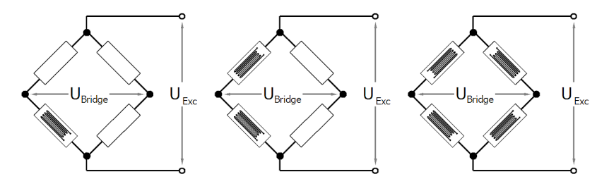 Fig.18: quarter, half, and full bridge
At this point, the three most important voltages in the bridge environment are defined:
- UExc:
- this is the feed voltage of the bridge as it comes from the measuring device or from an external source,
- usually in the range 1…12 V DC,
- it is fed to the bridge via supply line. Since current flows there, a voltage drop always occurs across the supply line; therefore, the bridge effectively only sees a voltage < UExc,
- other terms: UV, US, excitation, supply.
- USense:
- this is the bridge supply voltage as the measuring device “sees” it,
- usually in the range 1…12 V DC,
- without an extra sense supply line (e.g. 6‑wire operation of the full bridge) it is equal to UExc in the measuring device,
- if the bridge is operated with a sense line (full bridge: 6‑wire operation, half bridge: 5‑wire operation, quarter‑bridge: 3/4‑wire operation), USense returns to the measuring device from the bridge virtually current‑free and the measuring device knows the "true" UExc of the bridge,
- other terms: URef, reference, RemoteSense, feedback, compensation.
- UBridge:
- this is the very small differential bridge voltage "generated" by the load in the bridge, which is to be measured by the measuring device,
- it returns to the measuring device from the bridge virtually current‑free and is mostly in the range 1..50 mV, depending on the magnitude of UExc, the load and the bridge sensitivity,
- other terms: UD, UDifferential, signal, AI.
The measuring bridges can be operated with constant current, constant voltage, or also with AC voltage using the carrier frequency method.
| Measuring procedure The Beckhoff EL/KL335x terminals and the product group measurement technology ELM35/37xx, EPP35xx only support excitation with constant voltage. If excitation with AC is required, please contact Beckhoff sales. |
Full bridge strain gauge at constant voltage (ratiometric measurement)
Since the relative resistance change ΔR/R is low in relation to the nominal resistance R0, a simplified equation is given for the strain gauge in the Wheatstone bridge arrangement:
U D /U V = ¼ · (ΔR1‑ΔR2+ΔR3‑ΔR4)/R 0 .
ΔR/R usually has a positive sign in the case of elongation and a minus sign in the case of compression.
A suitable measuring instrument measures the bridge supply voltage UExc (or UV) and the resulting bridge voltage UBridge (or UD), and forms the quotients from both voltages, i.e. the ratio. After further calculation and scaling the measured value is output, e.g. in form of the effective mass in kg. Due to the division of UBridge and UExc the measurement is in principle independent of changes in the supply voltage.
If the voltages UBridge and UExc are measured simultaneously, i.e. at the same moment, and placed in relation to each other, this is referred to as a ratiometric measurement.
The advantage of this is that (with simultaneous measurement!) brief changes in the supply voltage (e.g. EMC effects) or a generally inaccurate or temporal unstable supply voltage likewise have no effect on the measurement.
A change in UV by e.g. 1 % creates the same percentage change in UD according to the above equation. Due to the simultaneous measurement of UD and UV the error cancels itself out completely during the division.
4‑wire vs. 6‑wire connection
With a constant voltage supply, the magnitude of the current can be quite considerable, e.g. 12 V / 350 Ω ≈ 34.3 mA. This leads not only to dissipated heat, wherein the specification of the strain gauge employed must not be exceeded, but possibly also to measuring errors in the case of inadequate wiring due to line losses not being taken into account or compensated.
In principle a full bridge can be operated with a 4‑conductor connection (two conductors for the supply UExc and two for the measurement of the bridge voltage UBridge).
If, for example, a 25 m copper cable (feed + return = 50 m) with a cross section q of 0.25 mm2 is used from the sensor up to the evaluating measurement module, this results in a line resistance of
RL = l/ (κ · q) = 50 m / (58 S · m/mm2 · 0.25 mm2 ) = 3.5 Ω
If this value remains constant, then the error resulting from it can be calibrated out. However, assuming a realistic temperature change of, for example, 30° the line resistance RL changes by
ΔRL = 30 K · 3.9 · 10‑3 1/K · 3.5 Ω = 0.41 Ω.
In relation to a measuring bridge with 350 Ω input impedance this means a measuring error of > 0.1 %.
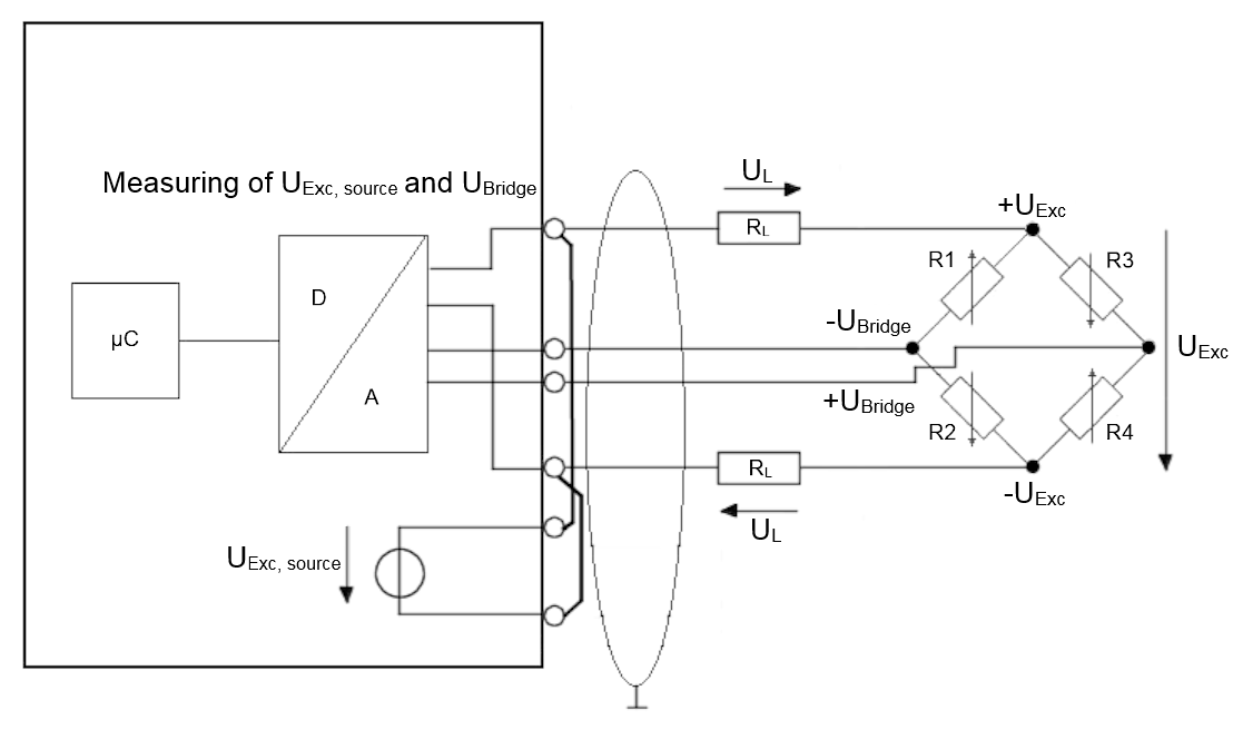 Fig.19: 4‑wire connection
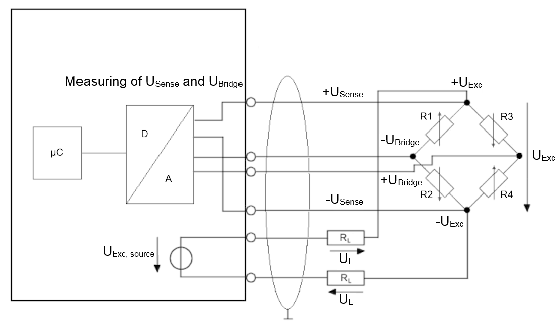 Fig.20: 6‑wire connection
 This can be remedied by a 6‑wire connection, in particular for precision applications.
The supply voltage UExc is thereby fed to the bridge (results in the pair of the current‑carrying conductors, the feed line). The supply voltage UExc is only measured with high impedance as reference voltage USense as the bridge voltage UBridge with two almost currentless return conductors each directly at the measuring bridge in the same way (often described as "Sense" input on measurement devices). Some measuring amplifiers then automatically increase the supply voltage thus far that the desired supply voltage is available at the bridge despite the potential difference on the supply line. In any case, the conductor‑related errors can be compensated by the back measurement of USense.
Since these are very small voltage levels of the order of mV and µV, all conductors should be screened.
Structure of a load cell with a strain gauge
One application of the strain gauge is the construction of load cells.
This involves gluing strain gauges (full bridges as a rule) to an elastic mechanical carrier, e.g. a double‑bending beam spring element, and additionally covered to protect against environmental influences.
The individual strain gauges are aligned for maximum output signals according to the load direction (two strain gauges in the elongation direction and two in the compression direction).
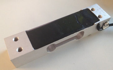 Fig.21: Example of a load cell
The most important characteristic data of a load cell
| Characteristic data Please enquire to the sensor manufacturer regarding the exact characteristic data! |
Nominal load Emax
Maximum permissible load for normal operation, e.g. 10 kg
Nominal characteristic value mV/V
The nominal characteristic describes the sensitivity of the load cell at nominal load Emax. This unit less value indicates the unbalance of the Wheatstone bridge, which, at supply voltage UExc, results in the output voltage UBridge.
An example: a nominal characteristic value 2 mV/V means that, with a supply of UExc = 10 V and at the full load Emax of the load cell, the maximum output voltage is
UBridge = 10 V · 2 mV/V = 20 mV. The nominal characteristic value is always a nominal value – a manufacturer’s test report is included with good load cells stating the characteristic value determined for the individual load cell, e.g. 2.0782 mV/V.
Accuracy class of a scale according to OIML R60
The accuracy class is indicated by a letter (A, B, C, D) and an additional digit, which encodes the scale interval d with a maximum number n max ( 1000), e.g. C4 means class C with a maximum of 4000 scale intervals. A division step is to be understood as the smallest possible/permissible unit with which weights can be differentiated. Smaller weight differences than the division unit can therefore not be clearly distinguished with the scale. The higher the quality of a weighing unit in terms of the components used and internal compensation elements, the finer its resolution.
The classes specify a maximum and minimum limit for scale intervals d:
- A: 50,000 – unlimited
- B: 5000 – 100,000
- C: 500 – 10,000
- D: 500 – 1000,
The scale interval nmax = 4000 states that, with a load cell with a resolution of Emin = 1 g, a calibratable set of scales can be built that has a maximum measuring range of 4000 · Emin = 4 kg. Since Emin is thereby a minimum specification, an 8 kg set of scales could be built – if the application allows – with the same load cell, wherein the calibratable resolution would then fall to 8 kg/4000 = 2 g. From another point of view the scale interval nmax is a maximum specification; hence, the above load cell could be used to build a set of scales with a measuring range of 4 kg, but a resolution of only 2000 divisions = 2 g, if this is adequate for the respective application. Also the classes differ in certain error limits related to non‑repeatability/creep/TC.
Accuracy class according to PTB
The European accuracy classes are defined in an almost identical way (source: PTB Braunschweig).
Class | Calibration value e | Minimum load Emin | Maximum load Emax | |
|---|---|---|---|---|
| Minimum value | Maximum value | ||
I Fine scales | 0.001 g < = e | 100 e | 50000 e | ‑ |
II Precision scales | 0.001 g < = e < = 0.05 g 0.1 g < = e | 20 e 50 e | 100 e 5000 e | 100000 e 100000 e |
III Commercial scales | 0.1 g < = e < = 2 g 5 g < = e | 20 e 20 e | 100 e 500 e | 10000 e 10000 e |
IIII Coarse scales | 5 g < = e | 10 e | 100 e | 1000 e |
It should be noted that a scale can usually only be used in a situation that is subject to calibration requirements with a considerably smaller scale interval than the data sheet indicates for an unregulated situation.
Minimum calibration value Emin
This indicates the smallest mass that can be measured without the maximum permissible error of the load cell being exceeded [RevT].
This value is represented either by the equation Emin = Emax / n (where n is an integer, e.g. 10000), or in % of Emax (e.g. 0.01%).
This means that a load cell with Emax = 10 kg has a maximum resolution of
Emin = 10 kg / 10000 = 1 g or Emin = 10 kg · 0.01% = 1 g.
Resolution of the scale / strain gauge vs resolution of the electronic recording
As described above, scales have a scale interval, i.e. a number of resolvable steps, e.g. 6000d. A 12 kg scale could therefore resolve to 2 g, which is 0.016 % or 166 ppm of the full-scale value.
On the other hand, there is the question of what electrical analog acquisition is necessary for such a scale, if it is to be utilized to the full. The answer is found in the following steps:
- The resolution of the analog value acquisition must in any case be equal to the scale graduation, or preferably greater. 6000d is approximately 212.5, so the analog value acquisition (ADC) must have at least 13 bitsunsigned, 14 bits signed if the analog input measures in bipolar mode (which is usually the case).
- However, 6000d means that the scale can unambiguously distinguish 6000 steps. This requirement must also be met by the analog value acquisition (weighing terminal). The measurement uncertainty of the weighing terminal is to be taken as the upper reference value for technically clearly distinguishable levels. So in this case it must be < 166 ppmfull-scale value for the 6000d scale to also meet a 6000d electronics.
- Ideally, the differential voltage Ubridge generated by the scale, e.g. 20 mV, should fully utilize the measuring range of the analog value acquisition to 100 %, i.e., up to the full-scale value (FSV)! Otherwise, this must be taken into account in the following calculation.
- It should be noted that the analog specification of the measurement uncertainty for Beckhoff analog products can vary depending on the terminal/box:
- with measurement error/uncertainty over the operating temperature range of the device, e.g. ±0.01%full-scale value at Tambient = 0...55 °C,
- or more precisely broken down in the extended analog characteristics: Basic accuracy @ Tambient = 23 °C and temperature coefficient of e.g. 10 ppm/K.
- If an even more precise consideration is required, the basic accuracy (measurement uncertainty at 23 °C) must be broken down further. The basic accuracy contains the four manufacturer-dependent elements: gain error, offset error, nonlinearity and repeatability.
- The offset error can easily be eliminated by a zero compensation (tare).
- Likewise, the gain error can be determined by adjustment with a calibration weight.
- The unavoidable remaining parameters are nonlinearity and repeatability. If these are provided in the Beckhoff device specification, they therefore represent the lowest limit for the possible "division" of the analog value acquisition. If, for example, the non-linearity over the whole measuring range, ELin = 50 ppm and the repeatability (at 23°C), ERep = 20 ppm, a scale with 14285d could be constructed from this (1/70 ppm).
- Note: This assumes, of course, that the temperature influence is eliminated by air conditioning and the noise of the analog recording is eliminated by (digital) filtering.
Minimum application range or minimum measuring range in % of rated load
This is the minimum measuring range or the minimum measuring range interval, which a calibratable load cell or scale must cover.
Example:
Above load cell Emax = 10 kg; minimum application range e.g. 40 % Emax.
The used measuring range of the load cell must be at least 4 kg. The minimum application range can lie in any range between Emin and Emax, e.g. between 2 kg and 6 kg if a tare mass of 2 kg already exists for structural reasons. A relationship between nmax and Emin is thereby likewise apparent: 4000 · 1 g = 4 kg.
There are other important characteristic values, which are for the most part self‑explanatory and need not be discussed further here, such as nominal characteristic value tolerance, input/output resistance, recommended supply voltage, nominal temperature range etc.
Parallel connection of strain gauges
It is usual to distribute a load mechanically to several strain gauge load cells at the same time. Hence, for example, the 3‑point bearing of a silo container on three load cells can be realized. Taking into account wind loads and loading dynamics, the total loading of the silo including the dead weight of the container can thus be measured. The mechanically parallel‑connected load cells are usually also electrically connected in parallel and to one measuring transducer, e.g. the EL3356. To this end the following must be observed:
- It is highly recommended that the load cells used are adjusted in the nominal characteristic value with a low tolerance, i.e. that they all have an approximately equal nominal characteristic value of e.g. 2 mV/V ±0.1%. If the load center and thus the load distribution among the load cells changes during successive weighings of the same weight, the final result remains the same. On the other hand, in the case of non-adjusted load cells with e.g. 2 mV/V ±10%, a variable load distribution due to a change in the force application point or weight center point leads to correspondingly variable weighing results.
- The input impedance of the load cells (as a rule, a few 10 Ω higher than the initial or nominal weight) must be such that the current supply capability of the supply (can be integrated into the transducer electronics) is not overloaded and
- the nominal characteristic value [mV/V] remains unchanged in the calculation, the rated load of the load cells must be added accordingly.
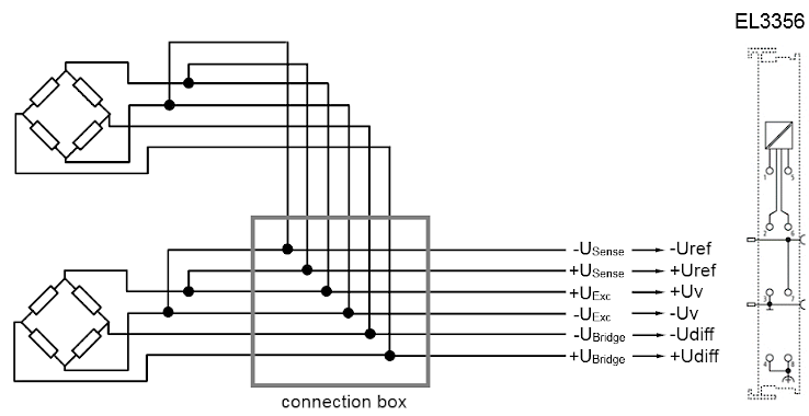 Fig.22: Parallel strain gauge
Shunt calibration
Notes on shunt calibration
Note: Not all Beckhoff strain gauge/bridge measuring devices support shunt calibration.
Shunt calibration refers to a procedure in which a known resistor is temporarily connected parallel to a bridge resistor. This is possible with all bridge circuits (quarter/half/full bridge); example for full bridge:
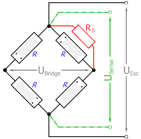 Fig.23: Shunt calibration
This electrically simulates a load on the measuring bridge; depending on the situation, a measuring signal step change between 0.1 and a few mV/V occurs. The interesting thing is that the step change, which is dependent on all the elements involved, is predictable.
Shunt calibration is used, for example, to
- find wire breakages or wiring faults during commissioning,
- simplify the initial calibration of the measuring setup: if the sensor cannot be loaded, the gain of the electrical measurement can be checked through the known detuning. Data acquisition can be even more extensive if the shunt is installed upstream in the sensor or in the bridge, rather than in the measuring device (in this case the Beckhoff measuring terminal),
- detection of resistance changes (that change the gain) in cables, plugs, full/half/quarter bridge during operation,
- compensate for actual line resistances during commissioning without having to install an (expensive) compensating line. For this purpose, the determined detuning is compared with the theoretically expected detuning and a corresponding gain correction factor is calculated in the PLC or terminal (however, a technically better way with regard to line resistances would be to use compensating lines, i.e. 3-wire mode for quarter bridge, 5-wire mode for half bridge, 6-wire mode for full bridge).
Shunt calibration procedure
- During commissioning, note the measured value at constant load, ideally without load.
- Close the shunt and note the difference to the previous measured value. A signal step change in [mV/V] should occur which corresponds to the precalculated value.
- During system operation the shunt calibration can be repeated regularly. The signal step change should not change significantly; if it does, it is an indication that electrically relevant components may have changed unintentionally.
Theoretically, the expected signal step change is based on the equation:

is 0.875 mV/V for R = 350 Ω and Rs = 100 kΩ.
Formulas and information on shunt calibration can be found in high-quality technical literature (Keil, Hoffmann) and can in some cases be obtained from bridge manufacturers (Vishay, HBM). However, it should be noted that the actual bridge design in commercially available measuring bridges/strain gauges often goes beyond the fundamentals described in simple standard works with R1...R4 = R. It is important to be aware of this, in order to be able to predict the signal step change [mV/V] during shunt calibration. Therefore, some aspects of actual measuring bridges are described below. Please note that the information is provided for general guidance only; for actual applications the user should discuss the finer details with the bridge manufacturer.
Input vs output impedance
Professionally manufactured measuring bridges/full bridges consist not only of the four bridge resistors R1, R2, R3, R4, but include a number of additional resistors and other sophisticated components, e.g. to compensate for temperature and non-linearity effects. The nominal or rated resistance of 120 or 350 Ω always refers to the output impedance (output resistance) of a bridge, i.e. the resistance that the measuring device sees at UBridge.
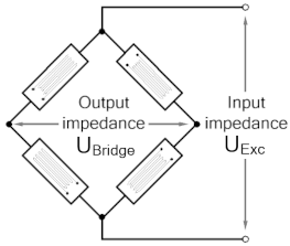 Fig.24: Measuring bridge with 4 bridge resistors
Theoretically the input impedance (input resistance) is the same, although in practice it is up to 25% larger than the output impedance, since, for example, with 350 Ω bridges, 2x approx. 32 Ω are often installed (for background on this see e.g. Stefan Keil, “Beanspruchungsermittlung mit Dehnmessstreifen”, 1995, Chap. 5.3), which are also detected by the sensor:
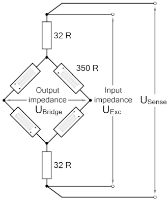 Fig.25: Measuring bridge with 4 bridge resistors and 2 additional resistors
This is irrelevant in non-shunt mode, in which the load on the supply is actually reduced. However, in shunt mode this information is crucial if the signal step change is to be predicted correctly. In addition, bridge designs vary greatly across the world, depending on the manufacturer and price range; in some cases bridges are asymmetrical in terms of UExc.
Line resistances
The shunt bridges supply lines, which means the influence of their resistance must also be known or measured in order to be able to predict the signal step change. Formulas and information on resistances of cables, connectors and switches can be found in the specialist literature, manufacturer data sheets and internet sources. Values in the range of a few 10s to 100 mΩ are common for short lengths.
Step change prediction
Due to the different characteristics of bridges and environments, no comprehensive values or formulas for step change prediction in [mV/V] can be provided here. More meaningful is specific calculation according to the respective conditions, taking into account the components that are essential for the shunt calibration. Common simulation tools are available for this purpose; further information can be requested via measurement@beckhoff.com.
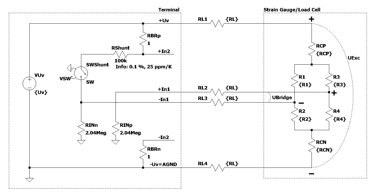 Fig.26: Example 1 - Comprehensive consideration of the 4-wire connection for an ELM350x
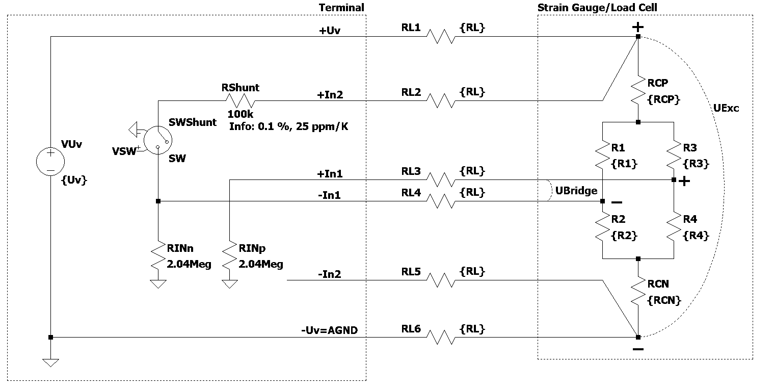 Fig.27: Example 2 - Comprehensive consideration of the 6-wire connection for an ELM350x
Sources of error/disturbance variables
Inherent electrical noise of the load cell
Electrical conductors exhibit so‑called thermal noise (thermal/Johnson noise), which is caused by irregular temperature‑dependent movements of the electrons in the conductor material. The resolution of the bridge signal is already limited by this physical effect. The rms value en of the noise voltage can be calculated by:
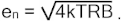
In the case of a load cell with R0 = 350 Ω at an ambient temperature T = 20 °C ( = 293K) and a bandwidth of the measuring transducer of 50 Hz (and Boltzmann constant k = 1.38 · 10‑23 J/K), the rms en = 16.8 nV. The peak‑peak noise epp is thus approx. epp ≈ 6.6 · en = 111 nV (thermal noise, 99.9 % interval of standard deviation).
Example:
For a bridge with 2 mV/V nominal characteristic value and supply of UExc = 5 V, this results in an output voltage UBridge_max = 5 V · 2 mV/V = 10 mV (for the nominal load) and therefore a maximum resolution of 10 mV / 111 nV = 90090 digits. Converted into bit resolution: ln(90090)/ln(2) ≈ 16 bits. Interpretation: a higher digital measuring resolution than 16 bits is thus inappropriate for such an analog signal in the first step. If a higher measuring resolution is used, then additional measures may need to be taken in the evaluation chain in order to gain a higher information content from the user- and noise superposition, e.g. hardware low‑pass filter or software algorithms.
This resolution applies alone to the measuring bridge without any further interferences. The resolution of the measuring signal can be meaningful increased by reducing the bandwidth of the measuring unit.
If the strain gauge is glued to a carrier (load cell) and wired up, both external electrical disturbances (e.g. thermovoltage at connection points) and mechanical vibrations in the vicinity (machines, drives, transformers and audible 50 Hz vibration due to magnetostriction etc.) can additionally impair the result of measurement.
Creep
Under a constant load, spring materials can further deform in the load direction. This process is reversible, but it generates a slowly changing measured value during the static measurement. In an ideal case the error can be compensated by constructive measures (geometry, adhesives).
Hysteresis
If even elongation and compression of the load cell take place, then the output voltage does not follow exactly the same curve, since the deformation of the strain gauge and the carrier runs different due to the adhesive and its layer thickness.
Temperature drift (inherent heating, ambient temperature)
Relatively large currents can flow in strain gauge applications. A full bridge with four 350 Ω resistors for example has a current consumption of I = UExc/R0 = 10 V / 350 Ω ≈ 28.6 mA. The power dissipation of the whole full bridge is thus PExc = U · I = 10 V · 28.6 mA = 286 mW. Depending on application (a cooling of the strain gauge takes place by heat dissipation into the carrier material) and carrier material a not insignificant error can arise that is termed apparent elongation. Therefore, the strain gauges on the sensor material are often counter‑compensated by the manufacturer.
Inadequate circuit technology
As already shown, a full bridge may be able (due to the system) to fully compensate hysteresis, creep and temperature drift. Wiring‑related measuring errors are avoided by the 6‑conductor connection.
Measuring body and natural frequency
In the dynamic measurement of forces and weights, the setup and some of the properties of the transducer play an essential part in the attainable dynamics. The natural frequency of the complete system limits the dynamics of the application and is influenced by the spring constant of the measuring body and the coupled mass. The softer the measuring body ( = larger deformation under nominal load), the lower the natural frequency. In the case of measuring transducers with rigid measuring bodies, too, the coupled mass must always be included if the natural frequency is to be determined.
Load cells are technologically similar to force transducers, but have a softer structure and are usually manufactured at optimized cost. Consequently, the recommendation for the mechanical setup is:
- use a rigid measuring transducer and the lightest possible mounted parts,
- the natural frequency of the system should be at least 2‑5 times higher than the measuring signal frequency (i.e. the dynamically moved test specimen from the application that is to be measured),
- Natural frequency specifications in data sheets apply only to the measuring transducer without mounted parts and are therefore not useable in the field. It is better to calculate with the nominal measuring path and masses of sensor plus mounted parts. The real natural frequency can be checked by means of a frequency analysis of the pulse response by FFT or manually by determining the period.
The natural frequency is to be calculated with:
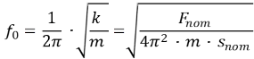 .
.
- f0 = natural frequency of the complete setup [Hz]
- Fnom = nominal force [N] or calculated nominal force by nominal load of the transducer [kg] and gravity of earth [m/s²]
- snom = nominal measuring path of the transducer (deformation under nominal load) [m]
- m = sum of dead weight and coupled mass [kg]
With Fnom = 450.5 N (50 kg nominal load and 9.81 m/s² gravity), snom = 0.18 mm, the resulting dependence on the mass, for example, is graphically:
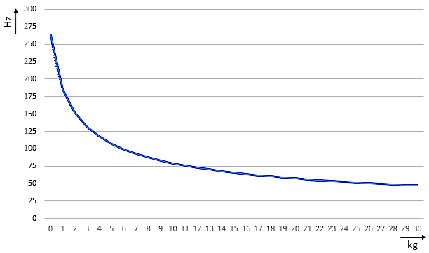 Fig.28: Natural frequency as a function of the total mass
Recommendations for strain gauge measurement with Beckhoff modules
- Electrical connection:
- Operation with an additional sense line for the bridge supply is recommended:
Full bridge in 6‑wire mode, half bridge in 5‑wire mode, quarter bridge in 3/4‑wire mode. - The use of full bridges instead of half or quarter bridges is generally recommended in order to achieve higher temperature stability and higher measuring accuracy.
- Selection of the feed voltage UExc:
- A feed voltage of 5 V has proven to be useful in many cases.
- In general it should be as high as possible within the permissible range according to the data sheet in order to achieve a large modulation of UBridge with the given nominal characteristic value [mV/V] and thus to maximize the electrical measuring range of the module (SNR increment).
- However, it should be considered that the heating of the bridge in the load cell increases quadratically with UExc to a first approximation. With high feed voltages and insufficient heat dissipation from the sensor to the machine, this can lead to massive drift effects after switching on.
- If necessary, select a bridge with a higher nominal parameter [mV/V] or a higher internal resistance [Ω].
- Selection of the nominal load of the weighbridge:
- It should be selected somewhat larger but as close as possible to the target load so that the mechanical and thus the electrical measuring range is utilized to the fullest extent possible.
- The overload capacity of the load cell must be observed. Fast weighing procedures in particular can lead to excessive mechanical stresses; nevertheless, as stated above, the bridge should not be over‑dimensioned (regarding Emax).
- The mechanical natural frequency of the load cell (in which the measuring bridge/strain gauge is installed!) or of the complete setup is to be considered in relation to the weighing procedures (number of product changes, product speed, product weights). If necessary, a significantly larger nominal load should be selected to the target load, because sensors with a higher nominal load have shorter nominal measuring paths and are thus mechanically more rigid. With a more rigid measuring body – usually the softest part of the entire setup – the natural frequency increases. As a result, the dynamics of the weighing procedure can be cleanly captured and measuring errors due to the natural oscillations of the weighing setup are avoided.
- Calibration/compensation of the bridge:
- Regular zero compensation (tare) is recommended.
- The tare effect should be observed in order to recognize a possibly damaged measuring bridge: the signal of a damaged measuring bridge drifts; it does not return to the original value after removal of the load.
- For the compensation of a gain error, a compensation point close to the target load should be selected during commissioning and if possible during operation, especially if this lies well below the nominal load (measurements in the partial load range).
- Possible filtering of the measurement, dynamic effects:
- In the case of fast sequential weighing procedures (several objects to be measured, e.g. products per second), it may be possible with adapted digital filters ‑ despite an obviously “poor” measuring signal ‑ to achieve a high measuring accuracy.
- Overshoot effects can often be observed for example, the pickup device for measurement objects (products) actually always moves mechanically (even if only in the µm range).
- The procedure of fast sequential weighing can also be dependent on the speed of which measurement objects (products) being moved over the weighting area; the filters for the measurement signal may then need to be dynamically adjusted.
- The optimal signal analysis is supported by Beckhoff with various products: flexible filters in the EtherCAT modules, TwinCAT filter designer, TwinCAT filter library, TwinCAT Analytics and so on.
References
Some organizations are listed below that provide the specifications or documents for the technological field of weighing technology:
- OIML (ORGANISATION INTERNATIONALE DE MÉTROLOGIE LÉGALE) www.oiml.org
- PTB ‑ Physikalisch‑Technischen Bundesanstalt www.ptb.de
- Arbeitsgemeinschaft Mess‑ und Eichwesen: www.eichamt.de
- WELMEC ‑ European cooperation in legal metrology www.welmec.org
- DKD ‑ Deutscher Kalibrierdienst www.dkd.eu
- Fachgemeinschaft Waagen (AWA) im Verband Deutscher Maschinen‑ und Anlagenbau VDMA www.vdma.org