Basic function principles
The measuring functions of the EP3356-0022 can be described as follows:
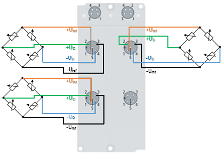
- The EP3356-0022 Analog Input Box are used to acquire the supply voltage to a load cell as a reference voltage, and the differential voltage that is proportional to the force acting on the cell.
- It is compulsory to connect a full bridge. If there is only a quarter or half bridge available, you have to add external auxiliary bridges. In this case you have to modify the nominal characteristic value.
- The reference and differential voltages are measured simultaneously
- Since the two voltages are measured at the same time, there is basically no need for a high-precision reference voltage with respect to the level. On changing the reference voltage, the differential voltage across the full bridge changes by the same degree. Therefore a stabilized reference voltage should be used that is subject to only low fluctuations (e.g. the EL95xx supply terminal)
- The change of the quotient of the differential and reference voltages corresponds to the relative force acting on the load cell.
- The quotient is converted into a weight and is output as process data.
- The data processing is subject to the following filtering procedures:
- the analog converter (ADC) integrates over 76 samples
- calculation of mean values in the averager (if activated)
- software filter IIR/FIR (if activated)
- The EP3356-0022 has an automatic compensation/self-calibration function. Default state: self-calibration activated, execution every 3 minutes
- errors in the analog input stages (temperature drift, long-term drift etc.) are checked by regular automatic calibration, and compensated to bring the measurement within the permitted tolerance range.
- the automatic function can be deactivated or activated in a controlled manner
- The EP3356-0022 can also be used as a 2-channel analog input box for voltage measurement.
- The EP3356-0022 has a timestamp function that can be activated through Distributed Clocks. The filter functionality is not available in Distributed Clocks mode.
General notes
- The measuring range should always be used as widely as possible in order to achieve a high measuring accuracy.
- Parallel operation of load cells is possible with the EP3356-0022. Please note:
- Load cells approved and calibrated by the load cell manufacturer for parallel operation should be used. The nominal characteristic values [mV/V], zero offset [mV/V] and impedance [Ω, ohm] are then usually adjusted accordingly.
- Load cell signals have a low amplitude and are occasionally very sensitive to electromagnetic interference. Considering the typical system characteristics and taking into account the technical possibilities, purposeful state-of-the-art EMC protective measures are to be taken. In the case of high electromagnetic interference levels, it may be helpful to additionally connect the cable screen before the box using suitable screening material.
- If the EP3356-0022 is to be used in Distributed Clocks mode:
- DC must be activated
- the Process data Timestamp must be activated. The filter functionality is not available then.
Signal flow diagram
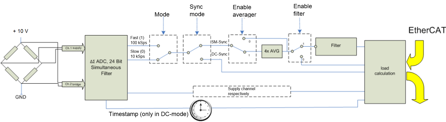
The EP3356-0022 processes the data in the following order:
- Hardware low-pass 10 kHz
- 2-channel simultaneous sampling at 10.5/105.5 kSps with 64-fold oversampling by delta-sigma (ΔΣ) converter and internal pre-filtration
- 4-fold averager (can be deactivated)
- Software filter (can be deactivated)
- Calculating the weight
 | Measurement principle of delta-sigma (ΔΣ) converter The measurement principle employed in the EP3356-0022, with real sampling in MHz range, shifts aliasing effects into a very high frequency range, so that normally no such effects are to be expected in the kHz range. |
Averager
In order to make use of the high data rates of the Analog-to-Digital converter (ADC) even with slow cycle times, a mean value filter is connected after the ADC. This determines the sliding mean value of the last 4 measured values. This function can be deactivated for each mode via the CoE object "Mode X enable averager".
Software filter
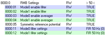
The EP3356-0022 is equipped with a digital software filter which, depending on its settings, can adopt the characteristics of a Finite Impulse Response filter (FIR filter), or an Infinite Impulse Response filter (IIR filter). The filter is activated by default as 50 Hz-FIR.
In the respective measuring mode the filter can be activated (0x8000:01, 0x8000:02) and parameterized (0x8000:11, 0x8000:12).
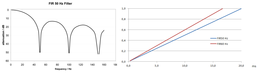
FIR 50/60 Hz
- The filter performs a notch filter function and determines the conversion time of the box. The higher the filter frequency, the faster the conversion time. A 50 Hz and a 60 Hz filter are available. Notch filter means that the filter has zeros (notches) in the frequency response at the filter frequency and multiples thereof, i.e. it attenuates the amplitude at these frequencies. The FIR filter operates as a non-recursive filter.
PDO filter
- The filter behaves like the 50/60 Hz FIR filter described above. However, the filter frequency can be adjusted here in 0.1 Hz steps by means of an output data object. The filter frequency range extends from 0.1 Hz to 200 Hz and can be reparameterised during operation. To do this the PDO 0x1601 (“RMB filter frequency”) must be displayed in the process data and the entry “PDO filter frequency” must be selected in the object 0x8000:11. This function allows the EP3356-0022 to suppress interference of a known frequency in the measuring signal. A typical application, for example, is a silo that is filled and weighed by a driven screw conveyor. The rotary speed of the screw conveyor is known and can be adopted into the object as a frequency. Thus mechanical oscillations can be removed from the measuring signal.
IIR-Filter 1 to 8
- The filter with IIR characteristics is a discrete time, linear, time invariant filter that can be set to eight levels (level 1 = weak recursive filter, up to level 8 = strong recursive filter). The IIR can be understood to be a moving average value calculation after a low-pass filter.
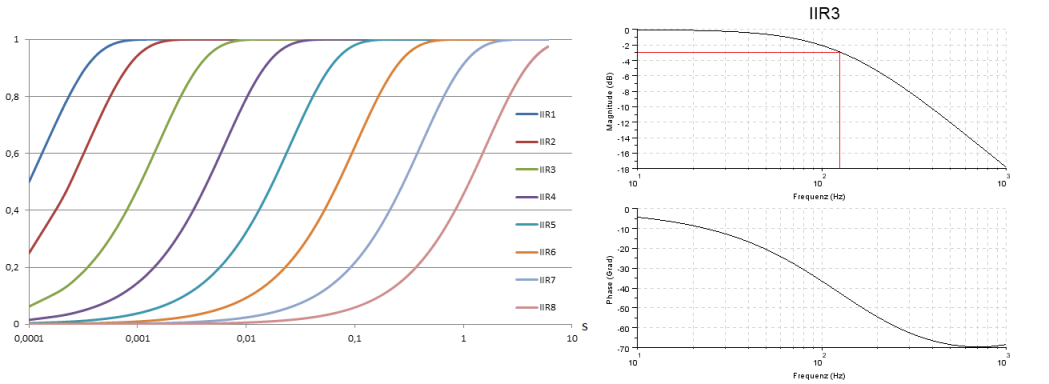
Overview of conversion times
Filter Settings | Value | PDO update time | Filter property | Limit frequency (-3 dB) [Hz] (typ.) | Comment | Rise time 10-90 % [s] (typ.) |
|---|---|---|---|---|---|---|
Filter deactivated | - | Cycle-synchronous,, min. 100 µs | - | - | - | - |
0 | FIR 50 Hz | 312.5 µs | 50 Hz notch filter | 22 Hz | Typ. conversion time 312.5 µs | 0.013 |
1 | FIR 60 Hz | 260.4 µs | 60 Hz notch filter | 25 Hz | Typ. conversion time 260.4 µs | 0.016 |
2 | IIR1 | Cycle-synchronous (up to min. 100 µs) | Low-pass | 2000 Hz | a0=1/21 = 0.5 | 0.0003 |
3 | IIR2 | Low-pass | 500 Hz | a0=1/22 = 0.25 | 0.0008 | |
4 | IIR3 | Low-pass | 125 Hz | a0=1/24 = 62.5e-3 | 0.0035 | |
5 | IIR4 | Low-pass | 30 Hz | a0=1/26 = 15.6e-3 | 0.014 | |
6 | IIR5 | Low-pass | 8 Hz | a0=1/28 = 3.91e-3 | 0.056 | |
7 | IIR6 | Low-pass | 2 Hz | a0=1/210 = 977e-6 | 0.225 | |
8 | IIR7 | Low-pass | 0.5 Hz | a0=1/212 = 244e-6 | 0.9 | |
9 | IIR8 | Low-pass | 0.1 Hz | a0=1/214 = 61.0e-6 | 3.6 | |
10 | Dynamic IIR | The filter changes dynamically between the filters IIR1 to IIR8 | ||||
11 | PDO Filter frequency | 1/PDO Value[Hz]*64 | Notch filter with adjustable frequency | ca. 0,443 * PDO Value [Hz] | - | - |
| Filter and cycle time If the FIR filters (50 Hz or 60 Hz) are switched on, the process data are updated maximally with the specified conversion time (see table). The IIR filter works cycle-synchronously. Hence, a new measured value is available in each PLC cycle. |
At which point the filters can be adjusted is described in the chapter “Object description and parameterization” for example under index 0x8000:12.
| IIR filter Differential equation: Yn = Xn * a0 + Yn-1 * b1 with a0 + b1 = 1 a0 = (see table), b1 = 1 - a0 |
Dynamic IIR Filter
The dynamic IIR filter automatically switches through the 8 different IIR filters depending on the weight change. The idea:
- The target state is always the IIR8-Filter, i.e. the greatest possible damping and hence a very calm measured value.
- In the input variable changes rapidly the filter is opened, i.e. switched to the next lower filter (if still possible). This gives the signal edge more weight and the measured value curve can follow the load quickly.
- If the measured value changes very little the filter is closed, i.e. switched to the next higher filter (if still possible). Hence the static state is mapped with a high accuracy.
- The evaluation as to whether a downward change of filter is required or whether an upward change is possible takes place continuously at fixed time intervals.
Parameterization takes place via the CoE entries 0x8000:13 and 0x8000:14. Evaluation takes place according to 2 parameters:
- The "Dynamic filter change time" object (0x8000:13) is used to set the time interval at which the existing signal is re-evaluated.
- Object 0x8000:14 is used to specify the maximum deviation that is permissible during this time without filter switching occurring.
Example:
The dynamic filter is to be adjusted in such a manner that a maximum slope of 0.5 digits per 100 ms (5 digits per second) is possible without the filter being opened. This results in a "calm" measured value. In the case of a faster change, however, it should be possible to immediately follow the load.
- Dynamic filter change time (0x8000:13) = 10 (equivalent to 100 ms)
- Object 0x8000:14 is used to specify the maximum deviation that is permissible during this time without filter switching occurring.
The measured value curve is shown below for a slower (left) and faster (right) change.

- Left: The scales are slowly loaded. The change in the weight (delta/time) remains below the mark of 0.5 digits per 100 ms. The filter therefore remains unchanged at the strongest level (IIR8), resulting in a low-fluctuation measured value.
- Right: The scales are suddenly loaded. The change in the weight immediately exceeds the limit value of 0.5 digits per 100 ms. The filter is opened every 100 ms by one level (IIR8 --> IIR7 --> IIR6 etc.) and the display value immediately follows the jump. After the removal of the weight the signal quickly falls again. If the change in the weight is less than 0.5 digit per 100 ms, the filter is set one level stronger every 100 ms until IIR8 is reached. The green line is intended to clarify the decreasing "noise level"
Calculating the weight
Each measurement of the analog inputs is followed by the calculation of the resulting weight or the resulting force, which is made up of the ratio of the measuring signal to the reference signal and of several calibrations.
YR = (UDiff / Uref) x Ai | (1.0) | Calculation of the raw value in mV/V |
YL = ( (YR – CZB) / (Cn – CZB) ) * Emax | (1.1) | Calculation of the weight |
YS = YL * AS | (1.2) | Scaling factor (e.g. factor 1000 for rescaling from kg to g) |
YG = YS * (G / 9.80665) | (1.3) | Influence of acceleration of gravity |
YAUS = YG x Gain - Tara | (1.4) | Gain and Tare |
Legend
Name | Designation | CoE Index |
|---|---|---|
UDiff | Bridge voltage/differential voltage of the sensor element, after averager and filter |
|
Uref | Bridge supply voltage/reference signal of the sensor element, after averager and filter |
|
Ai | Internal gain, not changeable. This factor accounts fort he unit standardisation from mV to V and the different full-scale deflections of the input channels |
|
Cn | Nominal characteristic value of the sensor element (unit mV/V, e.g. nominally 2 mV/V or 2.0234 mV/V according to calibration protocol) | |
CZB | Zero balance of the sensor element (unit mV/V, e.g. -0.0142 according to calibration protocol) | |
Emax | Nominal load of the sensor element | |
AS | Scaling factor (e.g. factor 1000 for rescaling from kg to g) | |
G | Acceleration of gravity in m/s^2 (default: 9.80665 ms/s^2) | |
Gain |
| |
Tare |
|
Conversion mode
The so–called conversion mode determines the speed and latency of the analog measurement in the EP3356-0022. The characteristics:
Mode | Meaning | typ. latency | typ. current consumption |
|---|---|---|---|
0 | High precision Analog conversion at 10.5 kSps (samples per second) Slow conversion and thus high accuracy | 7,2 ms | 70 % (see Technical data regarding nominal value) |
1 | High speed / low latency Analog conversion at 105.5 kSps (samples per second) Fast conversion with low latency | 0,72 ms | 100 % (see Technical data regarding nominal value) |
Due to the conversion principle of the EP3356-0022, the analog voltage is only available as a digital value after a defined time. This is shown in figure below.
A step signal 0->1 is applied to the input. The measured value is reached and readable within the defined accuracy after 7.2 ms or 0.72 ms, depending on the conversion mode 0/1. At this time the timestamp is also acquired in Distributed Clocks mode. In real operation a step signal is not normally connected, but rather a higher frequency but constant signal. The EP3356-0022 then maps the input signal with the corresponding latency for further processing, for which reason faster querying of the sampling unit at shorter intervals than the latency (EP3356-0022 allows up to 100 µs) makes sense for true-to-detail mapping of the analog input signal.
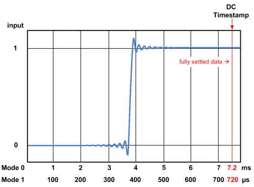
It is not possible to change the specified latency.
Beyond that the following are individually adjustable in each mode via CoE
- activation of the averager
- activation of the filter
- type of filter
Mode change
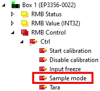
In particular for dynamic weighing procedures it may make sense to considerably change the measuring characteristic during the weighing procedure. For example, if a bulk material is filled by the sack within 5 seconds, a very open filter should initially be used so that the measured value quickly follows the fill level. During this phase it is of no importance that the measured value is very inaccurate and subject to high fluctuations. If the sack is >90 % full, filling must be slowed down and the loading must be followed with higher accuracy; the filter must be closed. Therefore the two conversion modes can be switched via the process data bit "Sample mode" in the EP3356-0022 in relation to the processing of the analog values.
The mode change takes about 30 ms, during which time the measured values are invalid and indicate this by the status byte.